Adding Text to Graphs by using Stata

Titles, captions and notes can be added to make graphs more self-explanatory. The default versions of titles and subtitles appear above the data region; notes (which might document the data source, for instance) and captions appear below. See Figure 3.7 for an example using title, caption and note. These defaults can be overridden, of course; type help title options for more information about placement of titles, or help textbox options for details concerning their content, including font size and color.

It also is possible to add text boxes at specified locations within the data region. For example, we might wish to annotate the plot of a time series, such as the historical ice-out dates on Lake Winnepesaukee, as done in Figure 3.26.

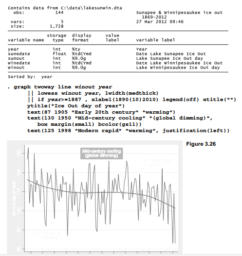
The basic graph in Figure 3.26 is a twoway line plot of Winnepesaukee ice-out day against years from 1887 through 2012. Overlaid on this is a second twoway plot showing a smooth lowess regression curve, drawn with a medium-thick line (lwidth(medthick)) to stand out. Lowess regression, explained in Chapter 8, provides a flexible approach to data smoothing that has several advantages over the better-known moving-average methods. The lowess curve in Figure 3.26 reveals multi-decade trends that underlie the jagged year-to-year variations.

Decadal trends on this lake broadly follow patterns of New Hampshire and global temperature over the same years (Hamilton et al. 2010a). Ice-out dates generally declined during a warming period of the late 19th and early 20th century. Slight cooling in mid-century, from the 1940s to the early 1970s, resulted in later ice-out dates. Globally, this period marks a time when sunlight reaching the surface was measurably dimmed by industrial pollution (Wild et al. 2007). During the warming from the mid-1970s on, Winnepesaukee ice-out dates more rapidly declined. The earliest recorded ice-out dates occurred in 2010 and 2012.

Three text boxes within the data region in Figure 3.26 note these climate episodes. They each contain two lines of text, broken within the text() options by separate sets of double quotes. The text() options specify y and x coordinates for the boxes; it often takes some experimenting to place them exactly where you want. The first box,

text(87 1905 “Early 20th century” “warming”)

is centered at y = 87 and x = 1905, with default attributes. The second box, at y = 130 and x = 1950, is shown surrounded by a visible border with small margin from the text. Border and background colors are specified as a medium gray, gs11.

text(130 1950 “Mid-century cooling” “(global dimming)”, box margin(small) bcolor(gs11))

The third box contains left-justified text.

text(125 1998 “Modern rapid” “warming”, justification(left))

See help textbox options and help colorstyle for more on controlling how text boxes look.

Source: Hamilton Lawrence C. (2012), Statistics with STATA: Version 12, Cengage Learning; 8th edition.