Regression with Random Intercepts by using Stata

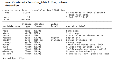
To illustrate xtmixed, we begin with county-level data on votes in the 2004 presidential election (Robinson 2005). In this election, George W. Bush (receiving 50.7% of the popular vote) defeated John Kerry (48.3%) and Ralph Nader (0.4%). One striking aspect of this election was its geographical pattern: Kerry won states on the West coast, the Northeast, and around the Great Lakes, while Bush won everywhere else. Within states, Bush’s support tended to be stronger in rural areas, whereas Kerry’s votes concentrated more in the cities. Dataset election_2004i contains election results and other variables covering most U.S. counties. A categorical variable notes census divisions (cendiv), which divide the U.S. into 9 geographical areas. Variables include the total number of votes cast (votes), the percent for Bush (bush), logarithm of population density (logdens) as an indicator of rural-ness, and other variables for the percent of county population belonging to ethnic minorities (minority), or adults having college degrees (colled).

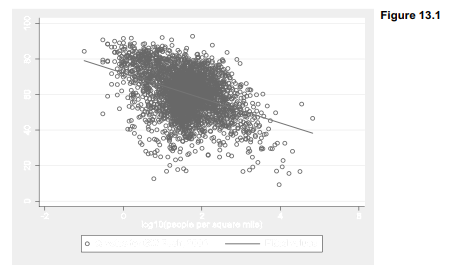
The percent voting for Bush declined as population density increased, as visualized by the scatterplot and regression line in Figure 13.1. Each point represents one of the 3,054 counties.

. graph twoway scatter bush

|| lfit bush logdens,

An improved version of this voting-density scatterplot appears in Figure 13.2. The logarithmic x-axis values have been relabeled (1 becomes “10”, 2 becomes “100,” and so forth) to make them more reader-friendly. Using votes as frequency weights for the scatterplot causes marker symbol area to be proportional to the total number of votes cast, visually distinguishing counties with small or large populations. Otherwise, analyses in this chapter do not make use of weighting. We focus here on patterns of county voting, rather than the votes of individuals within those counties.

. graph twoway scatter bush logdens [fw=votes], msymbol(Oh)

|| lfit bush logdens, lwidth(medthick)

|| , xlabel(-1 “0.1” 0 “1” 1 “10” 2 “100” 3 “1,000” 4 “10,000”, grid) legend(off)

xtitle(“Population per square mile”)

ytitle(“Percent vote for GW Bush”)

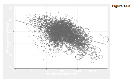
As Figure 13.2 confirms, the percent voting for George W. Bush tended to be lower in high- density, urban counties. It tended also to be lower in counties with substantial minority populations, or a greater proportion of adults with college degrees.

In mixed-modeling terms, we just estimated a model containing only fixed effects — intercept and coefficients that describe the sample as a whole. The same fixed-effects model can be estimated using xtmixed, with similar syntax.

Maximum likelihood (ML) is the default estimation method for xtmixed, but could be requested explicitly with the option ml. Alternatively, the option reml would call for maximum restricted likelihood estimation. See help xtmixed for a list of estimation, specification and reporting options.

The geographical pattern of voting seen in red state/blue state maps of this election are not captured by the fixed-effects model above, which assumes that the same intercept and slopes characterize all 3,041 counties in this analysis. One way to model the tendency toward different voting patterns in different parts of the country (and to reduce the problem of spatially correlated errors) is to allow each of the nine census divisions (New England, Middle Atlantic, Mountain, Pacific etc.) to have its own random intercept. Instead of the usual (fixed-effects) regression model such as

we could include not only a set of p coefficients that describe all the counties, but also a random intercept u₀, which varies from one census division to the next.

Equation [13.2] depicts the value ofy for the ith county and thejth census division as a function of X_i, x₂ and x₃ effects that are the same for all divisions. The random intercept u₀ j , however, allows for the possibility that the mean percent voting for Bush is systematically higher or lower among the counties of some divisions. That seems appropriate with regard to U.S. voting, given the obvious geographical patterns. We can estimate a model with random intercepts for each census division by adding a new random-effects part to the xtmixed command:

. xtmixed bush logdens minority colled || cendiv:

The upper section of an xtmixed output table shows the fixed-effects part of our model. This model implies nine separate intercepts, one for each census division, but they are not directly estimated. Instead, the lower section of the table gives an estimated standard deviation of the random intercepts (6.62), along with a standard error (1.60) and 95% confidence interval for that standard deviation. Our model is

If the standard deviation of u₀ appears significantly different from zero, we conclude that these intercepts do vary from place to place. That seems to be the case here — the standard deviation is more than four standard errors from zero, and its value is substantial (6.62 percentage points) in the metric of our dependent variable, percent voting for Bush. A likelihood-ratio test reported on the output’s final line confirms that this random-intercept model offers significant improvement over a linear regression model with fixed effects only (p ~ .0000).

Although xtmixed does not directly calculate random effects, we can obtain the best linear unbiased predictions (BLUPS) of random effects through predict. The following commands create a new variable named randintO, containing the predicted random intercepts, and then graph each census division’s random intercept in a bar chart (Figure 13.3).

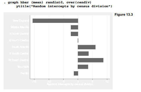
Figure 13.3 reveals that, at any given level of logdens, minority and colled, the percentage of votes going to Bush averaged about 15 points lower among New England counties, or more than 8 points higher in the W South Central (counties in Arkansas, Louisiana, Oklahoma and Texas), compared with the middle-of-the-road W North Central division.

Source: Hamilton Lawrence C. (2012), Statistics with STATA: Version 12, Cengage Learning; 8th edition.