Using Factor Scores in Regression by using Stata

Principal components and factor analysis often help to define new composite variables for further analysis. For example, the factor scores calculated by predict could become independent or dependent variables in subsequent regression analyses. To illustrate this process we turn to the survey dataset PNWsurvey211.dta.

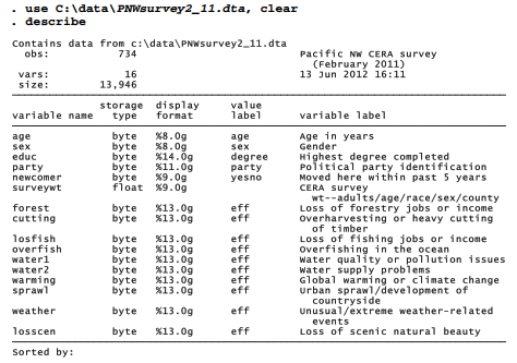
The 16 variables in this dataset represent a subset from a telephone survey of residents in a coastal region of the Pacific Northwest. This survey, conducted in February 2011, formed part of a series of regional surveys under the Community and Environment in Rural America (CERA) initiative (e.g., Hamilton et al. 2010b; Safford and Hamilton 2010).

Ten of the questions for this example, forest through losscen, ask whether particular environmental issues have had local effects. The questions go as follows.

I’m going to read a list of environmental issues that might be problems in some rural places. With regard to the place where YOU live, for each issue I’d like to know whether you think this has had no effect, had minor effects, or had major effects ON YOUR FAMILY OR COMMUNITY OVER THE PAST 5 YEARS?

Loss offorestry jobs or income?

Overharvesting or heavy cutting of timber?

Loss of fishing jobs or income?

Overfishing in the ocean?

Water quality and pollution issues?

Water supply problems?

Global warming or climate change?

Urban sprawl or rapid development of the countryside?

Unusual or extreme weather-related events?

Loss of scenic natural beauty?

For each question, respondents can say whether that issue had no effect, minor effects or major effects on their family or community.

Many respondents reported that loss of forestry or fishing jobs had major effects. Water supplies, urban sprawl and loss of scenic beauty were less immediate concerns for their region, as depicted in Figure 11.7. This overview graphic was created by drawing ten simple bar charts using catplot with analytical weights given by the surveywt variable ([aw = surveywt], see Chapter 4), then combining them into a single image with graph combine.

Does concern about these 10 environmental issues reflect a smaller number of underlying dimensions? Principal factoring with iterated communalities (ipf) identifies the underlying dimensions that best account for the pattern of correlations between variables.

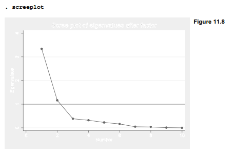
How many factors should we retain? Only the first two have eigenvalues above 1, although with principal factoring (unlike principal components) an eigenvalue-1 cutoff is sometimes viewed as too strict. A scree plot (Figure 11.8), however, visually confirms that after the first two factors, the remainder all have similar, low eigenvalues.

After further experiments with retaining and rotating two, three or more factors (not shown), it appears that two factors provide the most interpretable results — an important consideration. Once we decide to proceed with two factors, the next first step (because we are using iterated principal factoring) involves repeating the analysis with a factor(2) restriction.

Promax (oblique) rotation simplifies factor patterns while permitting some degree of correlation between the factors. Correlated factors will be statistically less parsimonious, because they have overlapping variance. However, they may be more realistic, if we view these factors as representing basic, not necessarily unrelated dimensions of environmental concern.

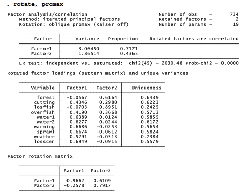
The survey questions about local effects of water quality or supply issues, global warming, extreme weather, urban sprawl and loss of scenic beauty all load much higher on factor 1. Concern about loss of forestry or fishing jobs load much higher on factor 2. Two items that involve both resource overuse and jobs, cutting and overfish, have roughly similar loadings on both factors. Based on these patterns we could interpret factor 1 as representing general environmental concern, and factor 2 as representing resource jobs concern. predict calculates factor scores, which are composite variables defined as sums of the variables’ standardized values, weighted by their factor score coefficients. The two new composite variables are named enviro and resjobs.

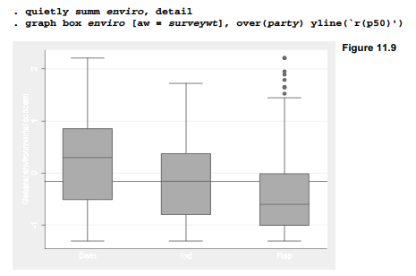
Social scientists constructing new composite variables look for evidence of their validity, or relation to what we think they measure. In this example one type of validity, face validity, is supported by the interpretable pattern of factor loadings. A second type, criterion validity, can be explored by testing whether the new variables correlate with other variables as theory or previous research predicts they should. For example, the single most robust finding from recent survey research on environmental concern in the U.S. has been the prevalence of ideological or political party-line effects. Box plots showing the distribution of scores on our general environmental-concern factor (enviro) over respondents’ political party clearly follow this expected pattern. A horizontal line in Figure 11.7 marks the overall median, taken from result r(p50) of a summarize, detail command with survey sampling weights used as analytical weights. Among respondents who identify themselves as Republican, those with high enviro scores appear as outliers.

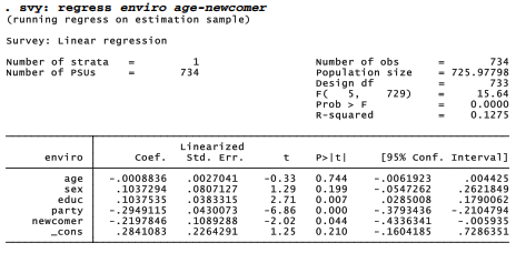
Other common findings reported by previous studies include effects from age, gender and education. The CERA researchers also had an interest in whether the environmental perceptions of rural-area newcomers differ from those of long-term residents. The regression below finds significant education, party and newcomer effects. Respondents who have more education, are Democrats or Independents, and have lived in this region for more than 5 years more often perceive local impacts from these environmental problems.

A similar regression with our resource-jobs concern factor resjobs finds that it is less affected by education or politics. Instead, age and newcomer status are the strongest predictors. Younger respondents, and those who moved into this area within the past five years, less often perceive impacts from the loss of fishing and forestry jobs.

Source: Hamilton Lawrence C. (2012), Statistics with STATA: Version 12, Cengage Learning; 8th edition.