What is panel data? and What is Panel Analysis?

What Is Panel Data?

In statistics and econometrics, panel data and longitudinal data are both multi-dimensional data involving measurements over time. Panel data is a subset of longitudinal data where observations are for the same subjects each time.

Time series and cross-sectional data can be thought of as special cases of panel data that are in one dimension only (one panel member or individual for the former, one time point for the latter). A literature search often involves time series, cross-sectional, or panel data. Cross-panel data (CPD) is an innovative yet underappreciated source of information in the mathematical and statistical sciences. CPD stands out from other research methods because it vividly illustrates how independent and dependent variables may shift between countries. This panel data collection allows researchers to examine the connection between variables across several cross-sections and time periods and analyze the results of policy actions in other nations.

A study that uses panel data is called a longitudinal study or panel study.

Advantages of using panel data

Panel data can be useful for professionals to collect, depending on what they’re studying. Here are some advantages of using panel data when conducting research studies:

Results in strong correlations: By combining information from the same test subjects over a long period of time, you can use panel data to correlate two or more variables with limited amounts of statistical uncertainty. For example, a study may collect annual data on the same 100 individuals’ levels of education and household incomes over a 15-year period. In this case, the researchers can use panel data to make a positive correlation between education and income.

Predicts future trends: Panel data allows you to predict how two or more variables are likely to interact in the future. It does this by tracking how the variables have historically behaved throughout the course of a study. For instance, researchers may be able to predict housing prices over the next five years by referencing panel data on city-specific housing prices from the past 20 years.

Collects data for future analysis: The panel data you collect now may provide insight for future studies related to variables included in your data. For instance, a current study on employment in the 1940s may use panel data collected during that decade to help researchers optimize their analysis. The 1940s data may include information like average wages, job types and unemployment rates, which can help current researchers better understand employment trends in the past.

Example of Panel data

Our panel data used in this article, that you can download here in Stata datasheet or Excel data, includes 434 year-observations of 62 provinces as entities of our sample; each province has 7 year-observations. These data were collected from the statistical yearbooks of Vietnam’s provinces during the period from 2010 to 2016; then cleaned by eliminating some missing-data provinces and year-observations.

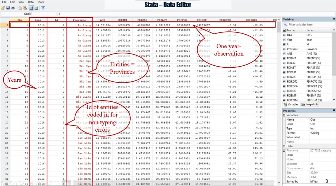
In this sample, “id” represents the entities as Vietnam provinces that we code them in number; and “year” represents the time variable (t). Note that you should make attention for assuring that all data of one thing such as one entity are coded exactly the same. If not, Stata will count as another thing or ignore it.

The objective of our research aims to study the relationship between foreign direct investment (FDI) and sustainability at provincial level in a developing host country as Vietnam for the period between the years of 2010 and 2016.

Here are the variables of our research; in which Dependent variable is the adjusted net savings that assess the sustainable development of Vietnam provinces. In total, we have 11 independent variables that are distinguished in three groups, including: 3 variables associated with the FDI inflow stocks; 5 variables associated with the employment in FDI sector, and 3 variables associated with the performance of FDI in provinces. And, 2 control variables are size and economic growth of province.

Panel data analysis

Panel (data) analysis is a statistical method, widely used in social science, epidemiology, and econometrics to analyze two-dimensional (typically cross sectional and longitudinal) panel data. The data are usually collected over time and over the same individuals and then a regression is run over these two dimensions. Multidimensional analysis is an econometric method in which data are collected over more than two dimensions (typically, time, individuals, and some third dimension).

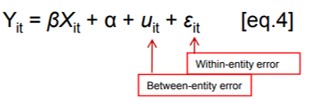
A common panel data regression model looks like Yit = α + βXit + εit, where Y is the dependent variable, X is the independent variable, α and β are coefficients, i and t are indices for individuals and time. The error εit is very important in this analysis. Assumptions about the error term determine whether we speak of fixed effects or random effects. In a fixed effects model, εit is assumed to vary non-stochastically over i or t making the fixed effects model analogous to a dummy variable model in one dimension. In a random effects model, εit is assumed to vary stochastically over i or t requiring special treatment of the error variance matrix.

Panel data analysis has three more-or-less independent approaches:

• independently pooled panels;
• fixed effects models or first differenced models;
• random effects models.

The selection between these methods depends upon the objective of the analysis, and the problems concerning the exogeneity of the explanatory variables.

Pooled OLS model

The Pooled OLS model applies the Ordinary Least Squares (OLS) methodology to panel data. This model assumes that there are no unobservable entity-specific effects, meaning that all entities in the data set are considered to have the same underlying characteristics. Consequently, αi is assumed to be constant across individuals and there is no dependence within individual groups (firms).

Y = α + βiXi + ε

Fixed-Effects Model

In panel data, we use fixed-effects model whenever we are only interested in analyzing the impact of variables that vary over time. This model is “designed to study the causes of changes within an entity. A time-invariant characteristic cannot cause such a change, because it is constant for each entity” (Kohler and Kreuter. 2008).

Fixed-effects model explores the relationship between independent variable and dependent variable within an entity as province in our empirical study. Each entity has its own individual characteristics as independent variables, that may or may not influence the dependent variable.

When using Fixed-effects model, we assume that something within the individual may impact or bias the independent variables and we need to control for this. This is the rationale behind the assumption of the correlation between entity’s error term and independent variables. Fixed-effects model remove the effect of those time-invariant characteristics so we can assess the net effect of the independent variables on the dependent one.

Another important assumption of the Fixed-effects model is that those time-invariant characteristics are unique to the individual and should not be correlated with other individual characteristics. Each entity is different therefore the entity’s error term and the constant (which captures individual characteristics) should not be correlated with the others. If the error terms are correlated, then Fixed-effects model is no suitable since inferences may not be correct, and we need to consider the random-effects model, this is the main rationale for the Hausman test.

The equation for the fixed effects model becomes:

Y_it = α_i + β_iX_it + u_it

Where:

• αi (i=1….n) is the unknown intercept for each entity (n entity-specific intercepts).
• Yit is the dependent variable (DV) where i = entity and t = time.
• Xit represents one independent variable (IV),
• β1 is the coefficient for that IV,
• uit is the error term

“The key insight is that if the unobserved variable does not change over time, then any changes in the dependent variable must be due to influences other than these fixed characteristics.” (Stock and Watson, 2003, p.289-290). “In the case of time-series cross-sectional data the interpretation of the beta coefficients would be “…for a given country, as X varies across time by one unit, Y increases or decreases by β units” (Bartels, Brandom, “Beyond “Fixed Versus Random Effects”: A framework for improving substantive and statistical analysis of panel, time-series cross-sectional, and multilevel data”, Stony Brook University, working paper, 2008). Fixed-effects will not work well with data for which within-cluster variation is minimal or for slow changing variables over time.

Another way to see the fixed effects model is by using binary variables. So the equation for the fixed effects model becomes:

You could add time effects to the entity effects model to have a time and entity fixed effects regression model:

Control for time effects whenever unexpected variation or special events my affect the outcome variable.

A note on fixed-effects that: “…The fixed-effects model controls for all time-invariant differences between the individuals, so the estimated coefficients of the fixed-efects models cannot be biased because of omitted time-invariant characteristics…[like culture, religion, gender, race, etc]. One side effect of the features of fixed-effects models is that they cannot be used to investigate time-invariant causes of the dependent variables. Technically, time-invariant characteristics of the individuals are perfectly collinear with the person [or entity] dummies. Substantively, fixed-effects models are designed to study the causes of changes within a person [or entity]. A time-invariant characteristic cannot cause such a change, because it is constant for each person.” (Kohler, Ulrich, Frauke Kreuter, Data Analysis Using Stata, 2nd ed., p.245).

Random-Effects Model

In panel data, the rationale behind random effects model is that: unlike the fixed-effects model, the variation across entities is assumed to be random and uncorrelated with the independent variables included in the model. So, “…the crucial distinction between fixed and random effects is whether the unobserved individual effect embodies elements that are correlated with the regressors in the model, not whether these effects are stochastic or not” (Green, 2008, p.183).

Random effects assume that the entity’s error term is not correlated with the independent variables which allow for time-invariant variables to play a role as independent variables.

If we have reason to believe that differences across entities have some influence on our dependent variable, then we should use random effects. An advantage of random effects is that: we can include time invariant variables (such as superficies of province). In the fixed effects model, these variables are absorbed by the intercept.

The random effects model is:

Random effects assume that the entity’s error term is not correlated with the predictors which allows for time-invariant variables to play a role as explanatory variables.

In random-effects, we need to specify those individual characteristics that may or may not influence the independent variables. The problem with this is that some variables may not be available therefore leading to omitted variable bias in the model.

RE allows to generalize the inferences beyond the sample used in the model.

Practical regression process

In panel data, the process of selecting the regression model for panel data (between Pooled OLS Model, Random-Effects Model and Fixed-Effects Model) is the one of Dougherty (2011).

Source: Dougherty (2011, p.421)

See more here how to choose the rigght model with Stata.