Probing the Interaction for Moderation with SEM Model

In our moderation example, we can see that the interaction is significant and positive, but we do not know much else about the interaction or ultimately how the moderator influences the relationship from the independent variable to the dependent variable. Next, we can “probe the interaction”, which means we are going to explore how the relationship from the independent variable to the dependent variable changes in different levels of the moderator.This is especially important when the independent variable has a weak relationship to the dependent variable, but the interaction of the moderator and the independent variable is significant. In those instances, we want to see where the relationship from the independent variable to the dependent variable changes when the moder- ator is at different levels.To accomplish this testing of different levels of a moderator, we are initially going to explore how to examine a moderator at low levels by creating a new “low level moderator” that is one standard deviation below the mean of the original moderator. Conversely, we are going to create a “high level moderator” test in which we examine the moderator at one standard devia- tion above the mean.This type of probing the interaction where you are choosing a specific point below and above the mean is called a spotlight analysis. It is also called a “pick-a-point approach” to moderation testing. Ultimately, probing the interaction gives you a better picture of how mod- eration is working in your model.

The first step is find the standard deviation for the moderator con- struct. In our previous moderator example, we needed to find the mean of the moderator. In that same output, the stand- ard deviation is provided as well (the Descriptives output). Based on that information, we know the standard deviation for the moderator of Friendliness is 1.37746. Let’s probe the interac- tion when the moderator is low.We need to form a new variable in the data set that represents the moderator at low levels.

Figure 7.6 Computing a Low Moderator Value to Probe the Interaction

Let’s call the new variable “LowFriend”. In the “Transform” menu in SPSS, we go to the “Com- pute Variable” function.We label our new construct and then take the mean centered compos- ite variable of the moderator of “centerFriend” and add the standard deviation to it. I know it seems odd to get the low moderator value by adding the standard deviation, but this is the necessary process to represent the low levels of the moderator. Once you have formed the “LowFriend” moderator, you need to create an interaction term with the low level moderator (LowFriend) and the mean centered independent variable of Adaptive Behavior (centerAdapt). Just to clarify, the interaction term will multiply “LowFriend” (mean centered moderator plus one standard deviation) by the mean centered independent variable “centerAdapt”. Let’s call the interaction term for the low moderator “Adapt_X_LowFriend”. Once you have formed this low moderator and interaction variable, we are ready to go back to AMOS and form a model for mod- eration testing. In AMOS, we will test this moderation the same way as we did before, except we are now using the low moderator and the interaction with the low moderator. To be efficient in creating the moderation model test, we can drag in the mean centered interaction of the Adaptive Behavior variable and low level moderator. We will also need to drag in the mean centered low level moderator variable. Lastly, we can leave the independent variable in the model as the original composite variable that was used in the first moderation test. Once you have the model drawn, we can run the analysis and then go to the Estimates link in the output.

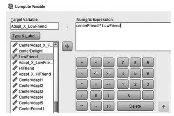
Figure 7.7 Forming an Interaction Term With Low Moderator Value

Figure 7.8 Moderation Test With Interaction Term  Including the Low Level of the Moderator

In the output, the only relationship we are concerned with is that of Adaptive Behavior to Customer Delight. We want to see how this relationship changes when low friendliness is included. Notice that the interaction results and moderator relationship to Customer Delight did not change from the original analysis.The results show that when the employee had a low degree of Friendliness, the relationship from Adaptive Behavior to Customer Delight is still significant but weaker. The original test had an unstandardized regression weight from Adap- tive Behavior to Customer Delight of .279, and now under low levels of the moderator, the relationship has weakened to .244.

Figure 7.9  Estimates Output With Low Moderator Interaction Term

We have examined the relationship when the moderator is low; let’s now examine when the moderator is strong or at high levels. In SPSS, let’s form a new variable called “HiFriend” which denotes high friendliness by the employee. We will take the mean centered variable of Friendliness, and this time we will subtract the standard deviation to get the high level moderator. After that, we will form an interaction term with “HiFriend” and the mean centered Adaptive Behav- ior construct “centerAdapt”. Let’s call the interaction term “Adapt_X_HiFriend”. Once these variables have been cre- ated and you have saved the SPSS file, you can drag in the high moderator variables in AMOS and then you are ready to run the analysis again.

Figure 7.10 Computing the High Level of the Moderator in SPSS

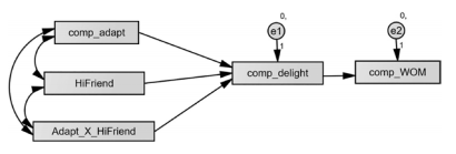
Figure 7.11 AMOS Model With Interaction Term Including the High Level of the Moderator

When we go to the Estimates link in the output, the relationship from Adaptive Behavior to Customer Delight is positive and significant again at high levels of the moderator. Hence, the construct of Friendliness is moderating the relationship of Adaptive Behavior to Customer Delight when Friendliness levels are weak and strong.When the moderator was high, the rela- tionship from Adaptive Behavior to Customer Delight strengthened even more than the initial test. The regression weight with high levels of the moderator was .315 compared to the first mean centered test of .279. By probing the interaction, you get a better picture of the relation- ship from the independent variable to the dependent variable in the presence of the moderator.

Figure 7.12 Estimates Output for Moderator at High Levels

With moderation testing, you want to interpret and present the unstandardized results of your analysis.The interaction term in a moderation test will not be properly standardized and is not interpretable (Frazier et al. 2004).Thus, you need to focus on the unstandardized results in testing for moderation.

Up to this point, we have discussed probing an interaction where you are choosing a specific point above and below the mean of the moderator to determine how the moderator influences the rela- tionship from the independent variable to the dependent variable.You can also use a floodlight analy- sis (Spiller et al. 2013) to probe an interaction where it does not look at a specific point above and below the mean; rather, it examines all possible points of the moderator to determine exactly where the interaction becomes significant. A floodlight analysis uses an approach that was initially intro- duced by Johnson and Neyman (1936).To examine the influence of all possible moderator values, a bootstrap is performed where you can see the regression weight of the interaction at different levels of the moderator.A confidence interval is also performed to let the reader know the level of signifi- cance at each level.The specific point where an interaction becomes significant is often referred to as the Johnson-Neyman point.You will also hear the term “regions of significance” to refer to a range of values that represent significance of the interaction of the moderator. Ultimately, the floodlight analysis is quite handy in telling you exactly what level of the moderator must be present to signifi- cantly influence the relationship from the independent variable to the dependent variable.

With having to calculate all possible values of the moderator, you can see where this would be impractical without some computational muscle. Many programs like SPSS, SAS, R, and others implement macros that can accomplish this analysis for you. I have even seen some researchers perform a quasi-floodlight analysis where they will pick numerous points below and above the mean of the moderator to assess the level of significance at different points.This is probably closer to a “pick-a-point” or spotlight analysis than a true floodlight analysis.

Probing an interaction via a floodlight analysis has grown in popularity because it allows a reader the ability to assess exactly where a relationship significantly changes in the presence of a moderator. Instead of examining a specific point, the reader now has the ability to see the entire range of the data. Saying that, you will often see a floodlight analysis presented in a graphical form to give the reader an easier interpretation of the data.

There is good news and bad news in regards to performing a floodlight analysis in AMOS. The bad news is that AMOS does not have a function that will calculate a floodlight analysis or even give you Johnson-Neyman points. The good news is that there are some researchers, such as James Gaskin, who are kind enough to develop and share a plugin for AMOS that will perform this analysis. A simple search on the internet will direct you to those plugins.To view an example of a floodlight analysis in graphical form, see Figure 7.13.

Figure 7.13 Example of Floodlight Analysis

Source: Thakkar, J.J. (2020). “Procedural Steps in Structural Equation Modelling”. In: Structural Equation Modelling. Studies in Systems, Decision and Control, vol 285. Springer, Singapore.