Sometimes you have more than one dependent variable that you want to analyze simultaneously. The GLM multivariate procedure allows you to analyze differences between levels of one or more (usually nominal level) independent variables, with respect to a linear combination of several dependent variables. One can also include normally distributed variables (covariates) as predictors of the linear combination of dependent variables. When you include both nominal variables and normally distributed variables as predictors, the analysis usually is referred to as MANCOVA (multivariate analysis of covariance).
11.1. Are there differences among the three father’s education groups on a linear combination of grades, math achievement, and visualization test? Also, are there differences between groups on any of these variables separately? Which ones?
Before we answer these questions, we will correlate the dependent variables to see if they are moderately correlated. To do this:
- Select Analyze → Correlate→Bivariate.
- Move grades in h.s., math achievement test, and visualization test into the Variables: box.
- Click on Options and select Exclude cases listwise (so that only participants with all three variables will be included in the correlations, just as they will be in the MANOVA).
- Click on Continue.
- Click on OK.
Compare your output with 11.1a.
Output 11.1a: Intercorrelations of the Independent Variables
CORRELATIONS /VARIABLES=grades mathach visual /PRINT=TWOTAIL NOSIG /MISSING=LISTWISE.
Correlations
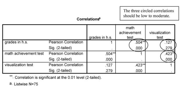
Interpretation of Output 11.1a
Look at the correlation table to see if correlations are too high or too low. One correlation is a bit high: the correlation between grades in h.s. and math achievement test (r = .504). Thus, we will keep an eye on it in the MANOVA that follows. If the correlations were .60 or above, we would consider either making a composite variable (in which the highly correlated variables were summed or averaged) or eliminating one of the variables.
Now, to do the actual MANOVA, follow these steps:
- Select Analyze → General Linear Model → Multivariate.
- Move grades in h.s., math achievement, and visualization test into the Dependent Variables
- Move father’s education revised into the Fixed Factor(s) box (see 11.1).
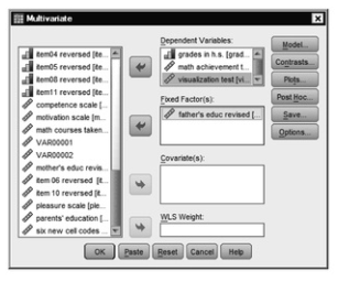
Fig. 11.1. Multivariate.
- Click on Options.
- Check Descriptive statistics, Estimates of effect size, Observed power, Parameter estimates, and Homogeneity tests (see 11.2). These will enable us to check other assumptions of the test and see which dependent variables contribute most to distinguishing between groups.
- Click on Continue.
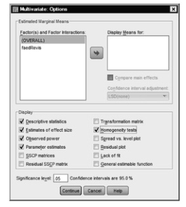
Fig.11.2.Multivariate options.
- Click on OK.
Compare your output with Output 11.1b.
Output 11.1b: One-Way Multivariate Analysis of Variance
GLMgrades mathach visual BY faedRevis /METHOD = SSTYPE(3) /INTERCEPT = INCLUDE
/PRINT = DESCRIPTIVE ETASQ OPOWER PARAMETER HOMOGENEITY /CRITERIA = ALPHA(.05)
/DESIGN = faedRevis.
General Linear Model
Interpretation of Output 11.1b
The GLM Multivariate procedure provides an analysis for “effects” on a linear combination of several dependent variables of one or more fixed factor/independent variables and/or covariates. Note that many of the results (e.g., Descriptive Statistics, Test of Between Subjects Effects) refer to the univariate tests.
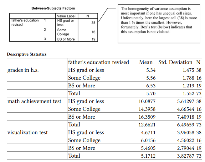
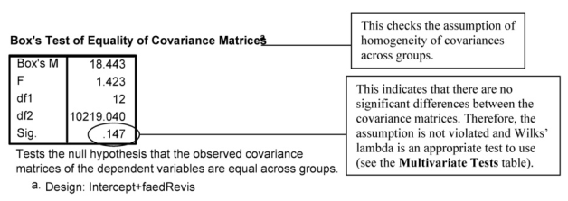
Box’s test of equality of covariance matrices tests whether the covariances among the three dependent variables are the same for the three father’s education groups. The Box test is strongly affected by violations of normality and may not be accurate. If Ns for the various groups are approximately equal, then the Box test can be ignored and Pillai’s trace used for the Multivariate statistic (below). Our largest group (N = 38) is 2.3 times larger than our smallest group (N = 16), so we should look at the Box test, which is not statistically significant (p = .147). Thus, the assumption of homogeneity of covariances is not violated. If the Box test had been statistically significant, we would have looked at the correlations among variables separately for the three groups and noted the magnitude of the discrepancies. None of the multivariate tests would be robust if Box’s test had been statistically significant and group sizes were very different.
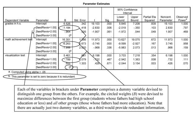
Interpretation of Output 11.1b continued In MANOVA, a linear combination of the dependent variables is created, and groups are compared on that variable. To create this linear combination for each participant, the computer multiplies the participant’s score on each variable by a weight (B), with the values of the weights being devised to maximize differences between groups. We see
these Bs in the next table (Parameter Estimates), so we can see how the dependent variables are weighted in the equation that maximally distinguishes the groups. Note that in the column under Parameter in this table, three variables are listed that seem new. These are the dummy variables that were used to test for differences between groups. The first one [faedrevis = 1.00] indicates differences between students whose fathers have a high school education or less and the other students whose fathers have more education. The second one [faedrevis = 2.00] indicates differences between students whose fathers have some college education and students in the other two groups. A third dummy variable would provide redundant information and, thus, is
not considered; there are k-1 independent dummy variables, where k = number of groups.
The next column, headed by B, indicates the weights for the dependent variables for that dummy variable. For example, in order to distinguish students whose fathers have a high school education or less from other
students, math achievement is weighted highest in absolute value (-6.263), followed by grades in h.s. (-1.184), and then visualization test (-.789). In all cases, students whose fathers have less education score lower than other students, as indicated by the minus signs. This table can also tell us which variables statistically significantly contributed toward distinguishing which groups, if you look at the sig column for each dummy variable. For example, both grades in high school and math achievement contributed statistically significantly toward discriminating group 1 (high school grad or less) from the other two groups, but no variables statistically significantly contributed to distinguishing group 2 (some college) from the other two groups (although grades in high school discriminates group 2 from the others at almost statistically significant levels). Visualization does not statistically significantly contribute to distinguishing any of the groups.
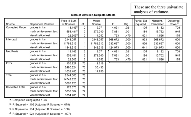
We can look at the ANOVA (Between-Subjects) and Parameter Estimates table results to determine whether the groups differ on each of these variables, examined alone. This will help us in determining whether multicollinearity affected results because if two or more of the ANOVAs are statistically significant, but the corresponding variables are not weighted much (examine the B scores) in the MANOVA, this probably is because of multicollinearity. The ANOVAs also help us understand which variables, separately, differ across groups.
Note that some statisticians think that it is not appropriate to examine the univariate ANOVAs. Traditionally, univariate Fs have been analyzed to understand where the differences are when there is a statistically significant multivariate F. One argument against reporting the univariate Fs is that it can be confusing to compare the univariate and multivariate results for two reasons. First, the univariate Fs do not take into account the relations among the dependent variables; thus, the variables that are statistically significant in the univariate tests are not always the ones that are weighted most highly in the multivariate test. Second, univariate Fs can be confusing because they will sometimes be statistically significant when the multivariate F is not because the multivariate is adjusted for the number of variables included. Furthermore, if one is using the MANOVA to reduce
Type I error by analyzing all dependent variables together, then analyzing the univariate Fs “undoes” this to a large extent, increasing Type I error. One method to compensate for this is to use the Bonferroni correction to adjust the alpha used to determine statistical significance of the univariate Fs. Despite these issues, most researchers elect to examine the univariate results following a statistically significant MANOVA to clarify which variables, taken alone, differ between groups.
Example of How to Write About Output 11.1
Results
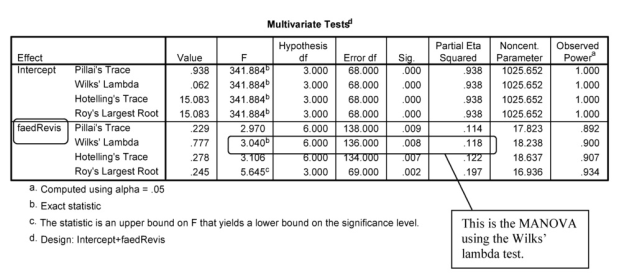
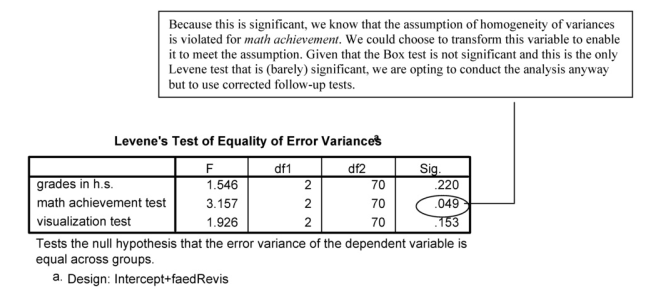
A multivariate analysis of variance was conducted to assess if there were differences between the three father’s education groups on a linear combination of grades in h.s., math achievement, and visualization test. (The assumptions of independence of observations and homogeneity of variance/covariance were checked and met. Bivariate scatterplots were checked for multivariate normality.) A statistically significant difference was found, Wilks’ A = .777, F(6, 136) = 3.04, p = .008, multivariate n2 = -12- Examination of the coefficients for the linear combinations distinguishing fathers’ education groups indicated that grades in high school and math achievement contributed most to distinguishing the groups. In particular, both grades in high school (0 = -1.18, p = .006, multivariate n2 = -10) and math achievement (0 = -6.26, p < .001, multivariate n2 = .17) contributed statistically significantly toward discriminating group 1 (high school grad or less) from the other two groups, but no variables statistically significantly contributed to distinguishing group 2 (some college) from the other two groups. Visualization did not contribute statistically significantly to distinguishing any of the groups.
Follow-up univariate ANOVAs indicated that both math achievement and grades in high school, when examined alone, were statistically significantly different for children of fathers with different degrees of education, F(2,70) = 7.88, p = .001 and F(2,70) = 4.09, p = .021, respectively.
Source: Leech Nancy L. (2014), IBM SPSS for Intermediate Statistics, Routledge; 5th edition;
download Datasets and Materials.
28 Mar 2023
15 Sep 2022
22 Sep 2022
14 Sep 2022
16 Sep 2022
28 Mar 2023