Inferential Statistics in SPSS: Interpreting the Results of a Statistical Test

In the following chapters, we present information about how to check assumptions, do the commands, interpret the previous statistics, and write about them. For each statistic, the program produces a number or calculated value based on the specific data in your study. They are labeled t, F, and so on, or sometimes just value.

Statistical Significance

The calculated value is compared to a critical value (found in a statistics table or stored in the computer’s memory) that takes into account the degrees of freedom, which are usually based on the number of participants. Based on this comparison, the program provides a probability value (called sig. for significance). It is the probability of a Type I error, which is the probability of rejecting the null hypothesis when it is actually true. Figure 6.3 shows how to interpret any inferential test once you know the probability level (p or sig.) from the computer or statistics table. In general, if the calculated value of the statistic (t, F, etc.) is relatively large, the probability or p is small (e.g., .05, .01, .001). If the probability is less than the preset alpha level (usually .05), we can say that the results are statistically significant or that they are significant at the .05 level. We can also say that the null hypothesis of no difference or no relationship can be rejected. Note that, using this program’s computer printouts, it is quite easy to determine statistical significance because the actual significance or probability level (p) is printed so you do not have to look up a critical value in a table. Because SPSS labels this p value or Sig., all of the common inferential statistics have a common metric, the significance level or Sig. Thus, regardless of what specific statistic you use, if the sig. or p is small (e.g., less than an alpha set at .05), the finding is statistically significant, and you can reject the null hypothesis of no difference or no relationship.

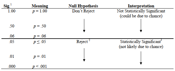
SPSS uses Sig. to indicate the significance or probability level (p) of all inferential statistics. This figure provides just a sample of Sig. values, which could be any value from 0 to 1.
.05 is the typical alpha level that researchers use to assess whether the null hypothesis should be rejected or not. However, sometimes researchers use more liberal levels (e.g., .10 in exploratory studies) or more conservative levels (e.g., .01).
Statistically significant does not mean that the results have practical significance or importance.

Fig.6.3. Interpreting inferential statistics using Sig.

Practical Significance Versus Statistical Significance

Students, and sometimes researchers, misinterpret statistically significant results as being practically or clinically important. But statistical significance is not the same as practical significance or importance. With large samples, you can find statistical significance even when the differences or associations are very small/weak. Thus, in addition to statistical significance, you should examine effect size. We will see that it is quite possible, with a large sample, to have a statistically significant result that is weak (i.e., has a small effect size.) Remember that the null hypothesis states that there is no difference or no association. A statistically significant result with a small effect size means that we can be very confident that there is at least a little difference or association, but it may not be of any practical importance.

Confidence Intervals

One alternative to null hypothesis significance testing (NHST) is to create confidence intervals. These intervals provide more information than NHST and may provide more practical information. For example, suppose one knew that an increase in reading scores of five points, obtained on a particular instrument, would lead to a functional increase in reading performance. Two different methods of instruction were compared. The result showed that students who used the new method scored significantly higher statistically than those who used the other method. According to NHST, we would reject the null hypothesis of no difference between methods and conclude that the new method is better. If we apply confidence intervals to this same study, we can determine an interval that contains the population mean difference 95% of the time. If the lower bound of that interval is greater than five points, we can conclude that using this method of instruction would lead to a practical or functional increase in reading levels. If, however, the confidence interval ranged from, say, 1 to 11, the result would be statistically significant, but the mean difference in the population could be as little as 1 point, or as big as 11 points. Given these results, we could not be confident that there would be a practical increase in reading using the new method.

Effect Size

A statistically significant outcome does not give information about the strength or size of the outcome. Therefore, it is important to know, in addition to information on statistical significance, the size of the effect. Effect size is defined as the strength of the relationship between the independent variable and the dependent variable, and/or the magnitude of the difference between levels of the independent variable with respect to the dependent variable. Statisticians have proposed many effect size measures that fall mainly into two types or families, the r family and the d family.

The r family of effect size measures. One method of expressing effect sizes is in terms of strength of association. The most well-known variant of this approach is the Pearson correlation coefficient, r. Using Pearson r, effect sizes always have an absolute value less than 1.0, varying between -1.0 and +1.0 with 0 representing no effect and +1 or -1 the maximum effect. This family of effect sizes includes many other associational statistics such as rho (r_s), phi (^), eta (n), and the multiple correlation (R).

The d family of effect size measures. The d family focuses on magnitude of difference rather than on strength of association. If one compares two groups, the effect size (d) can be computed by subtracting the mean of the second group (B) from the mean of the first group (A) and dividing by the pooled standard deviation of both groups. The general formula is below on the

left. If the two groups have equal ns, the pooled SD is the average of the SDs for the two groups. When ns are unequal, the formula below on the right is the appropriate one.

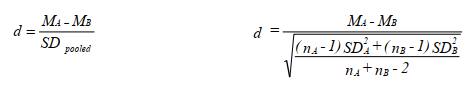
There are many other formulas for d family effect sizes, but they all express effect size in standard deviation units. Thus, a d of.5 means that the groups differ by one half of a pooled standard deviation. Using d, effect sizes usually vary from 0 to + or -1 but d can be more than 1.

Issues about effect size measures. Unfortunately, as just indicated, there are many different effect size measures and little agreement about which to use. Although d is the most commonly discussed effect size measure for differences between groups, it is not available on SPSS outputs. However, d can be calculated by hand from information in the printout, using the previous appropriate formula. The correlation coefficient, r, and other measures of the strength of association, such as phi (^), eta² (n2), and R,² are available in the outputs if requested.

There is disagreement among researchers about whether it is best to express effect size as the unsquared or squared r family statistic (e.g., r or r²). The squared versions have been used because they indicate the percentage of variance in the dependent variable that can be predicted from the independent variable(s). However, some statisticians argue that these usually small percentages give you an underestimated impression of the strength or importance of the effect. Thus, we (like Cohen, 1988) decided to use the unsquared statistics (r, (|>, n, and R) as our r family indexes.

Relatively few researchers reported effect sizes before 1999 when the APA Task Force on Statistical Inference stated that effect sizes should always be reported for your primary results (Wilkinson & The Task Force, 1999). The 5th edition (APA, 2001) adopted this recommendation of the Task Force so, now, most journal articles discuss the size of the effect as well as whether or not the result was statistically significant.

Interpreting Effect Sizes

Assuming that you have computed an effect size measure, how should it be interpreted? Based on Cohen (1988), Table 6.5 provides guidelines for interpreting the size of the “effect” for five common effect size measures: d, r, (|>, R and n.

Note that these guidelines are based on the effect sizes usually found in studies in the behavioral sciences and education. Thus, they do not have absolute meaning; large, medium, and small are only relative to typical findings in these areas. For that reason, we suggest using “larger than typical” instead of large, “typical” instead of medium, and “smaller than typical” instead of small. The guidelines do not apply to all subfields in the behavioral sciences, and they definitely do not apply to fields, designs, or contexts where the usually expected effects are either larger or smaller. It is advisable to examine the research literature to see if there is information about typical effect sizes on the topic and adjust the values that are considered typical accordingly.

Table 6.5. Interpretation of the Strength of a Relationship (Effect Sizes)

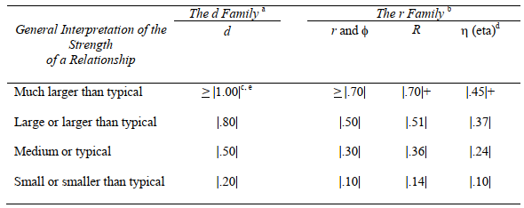
a d values can vary from 0.0 to + or — infinity, but d greater than 1.0 is relatively uncommon.

^b r family values can vary from 0.0 to + or – 1.0, but except for reliability (i.e., same concept measured twice), r is rarely above .70. In fact, some of these statistics (e.g., phi) have a restricted range in certain cases; that is, the maximum phi is less than 1.0.

^c We interpret the numbers in this table as a range of values. For example, a d greater than .90 (or less than -.90) would be described as “much larger than typical,” a d between, say, .70 and .90 would be called “larger than typical,” and d between, say, .60 and .70 would be “typical to larger than typical.” We interpret the other three columns similarly.

^d Partial etas are multivariate tests equivalent to R. Use R column.

^e Note. | | indicates absolute value of the coefficient. The absolute magnitude of the coefficient, rather than its sign, is the information that is relevant to effect size. R and n usually are calculated by taking the square root of a squared value, so that the sign usually is positive.

Cohen (1988) provided research examples of what he labeled small, medium, and large effects to support the suggested d and r family values. Most researchers would not consider a correlation (r) of .5 to be very strong because only 25% of the variance in the dependent variable is predicted. However, Cohen argued that a d of .8 (and an r of .5, which he showed are mathematically similar) are “grossly perceptible and therefore large differences, as (for example, is) the mean difference in height between 13- and 18-year-old girls” (p. 27). Cohen stated that a small effect may be difficult to detect, perhaps because it is in a less well-controlled area of research. Cohen’s medium size effect is “… visible to the naked eye. That is, in the course of normal experiences, one would become aware of an average difference in IQ between clerical and semi-skilled workers …” (p. 26).

Effect size and practical significance. The effect size indicates the strength of the relationship or magnitude of the difference and thus is relevant to the issue of practical significance. Although some researchers consider effect size measures to be an index of practical significance, we think that even effect size measures are not direct indexes of the importance of a finding. As implied earlier, what constitutes a large or important effect depends on the specific area studied, the context, and the methods used. Furthermore, practical significance always involves a judgment by the researcher and/or the consumers (e.g., clinicians, clients, teachers, school boards) of research that takes into account such factors as cost and political considerations. A common example is that the effect size of taking daily aspirin on heart attacks is quite small but the practical importance is high because preventing heart attacks is a life or death matter, the cost of aspirin is low, and side effects are uncommon. On the other hand, a curriculum change could have a large effect size but be judged impractical because of high costs and/or extensive opposition to its implementation.

Confidence intervals of the effect size. Knowing the confidence interval around an effect size can provide information useful to making a decision about practical significance or importance. If the confidence interval is narrow, one would know that the effect size in the population is close to the computed effect size. On the other hand, if the confidence interval is large (as is usually the case with small samples) the population effect size could fall within a wide range, making it difficult to interpret the computed effect size for purposes of estimating practical significance. Similar to the example described earlier, if the lower bound of the confidence interval was more than a minimum effect size agreed to indicate a practically significant effect, one could then be quite confident that the effect was important or practical. Unfortunately, SPSS does not provide confidence intervals for effect size measures and it is not easy to compute them by hand.

Steps in Interpreting Inferential Statistics

When you interpret inferential statistics, we recommend:

Decide whether to reject the null hypothesis. However, that is not enough for a full interpretation. If you find that the outcome is statistically significant, you need to answer at least two more Figure 6.4 summarizes the steps described later about how to more fully interpret the results of an inferential statistic.
What is the direction of the effect? Difference inferential statistics compare groups so it is necessary to state which group performed better. We discuss how to do this in Chapters 9 and 10. For associational inferential statistics (e.g., correlation), the sign is very important, so you must indicate whether the association or relationship is positive or negative. We discuss how to interpret associational statistics in Chapters 7 and 8.

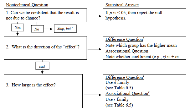
^a If you have a small sample (N), it is possible to have a nonsignificant result (it may be due to chance) and yet a large effect size. If so, an attempt to replicate the study with a larger sample may be justified.

^b If there are three or more means or a significant interaction, a post hoc test (e.g., Tukey) will be necessary for complete interpretation.

^c Interpretation of effect size is based on Cohen (1988) and Table 6.5. A “large” effect is one that Cohen stated is “grossly perceptible.” It is larger than typically found but does not necessarily explain a large amount of variance. You might use confidence intervals in addition to or instead of effect sizes.

Fig.6.4. Steps in the interpretation of an inferential statistic.

What is the size of the effect? It is desirable to include the effect size and/or the confidence interval in the description of all your results or at least provide the information to compute them. Unfortunately, SPSS does not always provide effect sizes and confidence intervals, so for some statistics we have to compute or estimate the effect size by hand, or use an effect size calculator, several of which are available online.
Although not shown in the Fig. 6.4, the researcher or the consumer of the research should make a judgment about whether the result has practical or clinical significance or importance. To do so, they need to take into account the effect size, the costs of implementing change, and the probability and severity of any side effects or unintended consequences.

Source: Morgan George A, Leech Nancy L., Gloeckner Gene W., Barrett Karen C.

(2012), IBM SPSS for Introductory Statistics: Use and Interpretation, Routledge; 5th edition; download Datasets and Materials.