You can test null hypotheses about the effects of both between-groups factors and within-subjects factors with a Mixed ANOVA using the General Linear Model procedure. You can investigate interactions between factors as well as the effects of individual factors on a dependent variable.
Repeat Problem 10.1 except add gender to see if there are any gender differences as well as product differences and if there is an interaction between gender and product. Is gender a between-groups/subjects or within-subjects variable? The answer is important in how you compute and interpret the analysis.
- Are there gender as well as product differences? Is there an interaction between gender and product?
- Click on Analyze → General Linear Model → Repeated Measures to get 10.3 again.
- In the Repeated Measures Define Factor(s) window ( 10.3), you should see product (4) in the top big box. If so, click on Define (if not repeat the steps for Problem 10.1).
- Then move gender to the Between-Subjects Factor(s) box ( 10.4).
- Click on Contrasts to get 10.5.
- Click on product(polynomial) under Factors.
- Be sure that Repeated is listed under Contrast, then click Change. This will make it say product (Repeated).
- Click Continue.
- Click on Options and be sure that Descriptive Statistics, Estimates of effect size, and Observed power are checked.
- Click Continue.
- Click on Plots.
- Move gender to the Separate Lines box and product to the Horizontal Axis
- Click
- Click on OK.
Compare your syntax and output with Output 10.3.
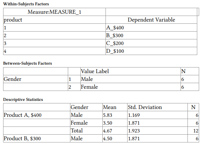
Output 10.3: Mixed ANOVA: Product by Gender
GLM A_$400 B_$300 C_$200 D_$100 BY gender /WSFACTOR=Product D
Repeated
/METHOD=SSTYPE(3)
/PRINT=DESCRIPTIVE ETASQ OPOWER
/CRITERIA=ALPHA(.05)
/WSDESIGN=product
/DESIGN=gender.
General Linear Model
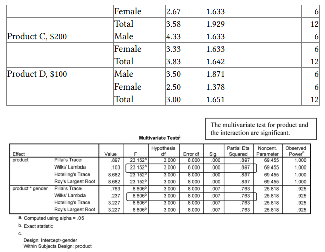
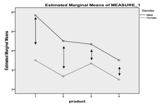
Note that although the general shape of the curves are similar for males and females, there seems to be a greater difference between males’ and females’ ratings of the less expensive products relative to the more expensive ones.
Interpretation of Output 10.3
Most of these tables are similar in format and interpretation to those in
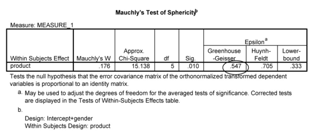
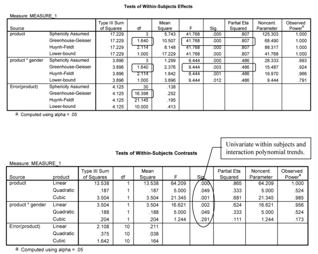
Output 10.1. However, the addition of gender as a between-subjects independent variable makes the last table meaningful and adds an interaction (product * gender) to both the Multivariate Tests table and the univariate (Tests of Within-Subjects Effects) tables. Both multivariate and univariate tables indicate that (as in Output 10.1) there are differences among the four products, with a very large effect size (partial eta). Again, one should interpret the Greenhouse-Geisser univariate test with corrected degrees of freedom given the lack of sphericity. In addition, the interaction of product and gender is significant according to both univariate and multivariate tests. This means that the downward overall trend for all subjects is somewhat different for males and females. The figure shows that males seem to rate the two inexpensive products more highly than do females, whereas the difference between ratings of males and females isn’t as great for the two most expensive products. Recall that the Tests of Within-Subjects Contrasts table shows whether the four product means are significantly like a straight line (linear effect), a line with one change in direction (quadratic), and a two-bend line (cubic). Again, there are significant linear and cubic trends, but now the quadratic trend is also significant. For males, there is a linear decline in ratings from Product A (5.83) to Product D (3.50). For females, Product B has a lower mean (2.67) than Product A (3.50) and Product C (3.33) producing the cubic trend. And then the mean for Product D (2.50) is again lower, which produces the quadratic trend. Moreover, the linear and quadratic trends are significant for the interaction between product and gender.
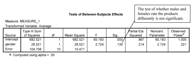
The last table indicates that the males and female product rating do not statistically significantly differ (p = .13). However, the observed power is very low (.32) so we did not have enough power to detect the gender difference even though the effect size is large, eta = .46 (7.214). Remember that there were only six males and six females in this small sample.
Note that if we had three groups, instead of just males and females, for our between-groups variable and if the ANOVA had been significant, we would have used a between-groups post hoc test for this effect. SPSS provides the same wide variety of post hoc multiple comparisons for the Between- Subjects Effects that were available for one-way ANOVA and factorial
ANOVAs, including the Tukey HSD and Games Howell.
Example of How to Write About Output 10.3
Results
A mixed ANOVA was conducted to assess whether there were gender and product differences in product ratings. (The following assumptions were tested: (a) independence of observations, (b) normality, and (c) sphericity. Independence of observations and normality were met. The assumption of sphericity was violated. Thus, the Greenhouse-Geisser epsilon was used to correct degrees of freedom.) Results indicated a statistically significant main effect of product, F(1.64, 16.4) = 41.77, p < . 001, partial eta2 = .807, but not of gender, F(1, 10) = 2.72, p = .13, partial eta2 = .214. However, the product main effect was qualified by a statistically significant interaction between product and gender, F(1.64, 16.40) = 9.44, p = .003, partial eta2 = .486. Table 10.1 provides the means and standard deviations for product ratings by gender, and Figure 10.9 graphically represents the interaction between product and gender. Inspection of the figure suggests that males seem to rate the two inexpensive products more highly than do females; whereas the difference between ratings of males and females is less pronounced for the two most expensive products.
Source: Leech Nancy L. (2014), IBM SPSS for Intermediate Statistics, Routledge; 5th edition;
download Datasets and Materials.
16 Sep 2022
29 Mar 2023
15 Sep 2022
30 Mar 2023
30 Mar 2023
28 Mar 2023