Problem 13.3: Mixed Models Analysis after Imputed Data with SPSS

We will now conduct a mixed model analysis on the imputed data. This analysis is appropriate because our data involve repeated measures that are arrayed as multiple lines for each participant. The Mixed Models procedure is one that is set up in SPSS to readily read and use imputation datasets. We have discussed this type of analysis in much greater detail in Chapter 12, so in this chapter, we will not interpret all parts of the analysis. Our main goal in this chapter is to show an analysis that can be run with an imputation dataset and how the output indicates results involving imputation. Please see Chapter 12 for more information about this procedure. Some programs can be run using imputation datasets, and others cannot. Mixed model analysis is one that can be used and which can take into account the within-subjects variable, time.

• First, make sure that your data will be analyzed separately for each imputation dataset by specifying that the data should be split based on imputation number. To do this:
• Click on Data^Split File. You should see a window similar to A.10 in Appendix A.
• Click on Compare groups. Move Imputation number into the Groups based on
• Now click on Analyze^Mixed Models ^Linear.
• In the first window, move Patient number into the Subjects box, Time into the Repeated box, and select AR(1) from the drop-down menu for Repeated Covariance Type.
• Click on Continue.
• In the next window, move weight into the Dependent Variable box, time in the Factors box, and binge, mood, and preo into the Covariates
• Click on Statistics, and check Parameter estimates, Tests for covariance parameters, and Contrast coefficient matrix. Click on Continue. Then click on OK in the window that you see next.
• Your output should look like Output 13.3, except that we have omitted some parts to save space.

Output 13.3: Analysis of Imputed Data with Mixed Models

Interpretation of Output 13.3

The Information criteria table indicates goodness of fit of the model with the data, with smaller numbers indicating better fit. Note that the imputed data, for each of the five imputations shown, have somewhat poorer fits to the data. However, we will see below that the results of the tests predicting weight from the time various predictors are highly significant for the imputed models. Remember that we only have provided results for the first 5 imputations.

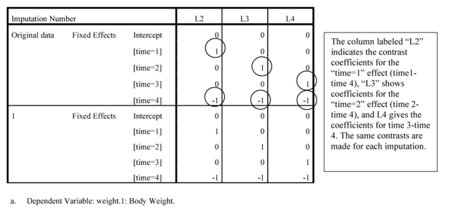
In the next table, coefficients are given for the contrasts between levels of time. Dummy variables are created in which each level of time is contrasted with time 4. Thus, [time=1] contrasts the first time point with time 4, [time=2] contrasts time 2 with time 4, and [time=3] contrasts time 3 with time 4. There can only be 3 contrasts because there are only 3 degrees of freedom for 4 levels of the time variable.

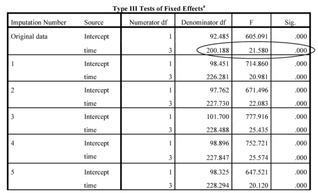
Interpretation of Output 13.3 (continued) Note that results are significant for the effect of time on Weight for all imputations (only the first 5 are presented here) and time is analyzed in the same way for all imputations.

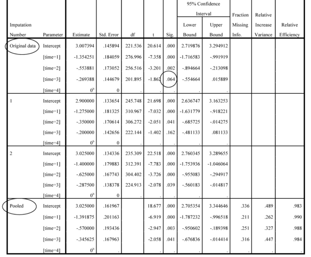
Interpretation of Output 13.3 continued The Estimates of Fixed Effects results are provided for each imputation, as well as original and pooled results. Because an imputation dataset was used, three new columns are produced, indicating (on the Pooled row only) amount of missing data, increase in variance once missing data were imputed, and relative efficiency once data were imputed. The Fraction Missing Info column is an estimate of amount of missing data, based on the relative increase in variance from adding the imputed data. Relative increase in variance is the ratio of between-imputation to within imputation variance of the regression coefficient. Estimating missing data from existing data leads to an underestimate of the true variance, so between imputation variance is used as an estimate of this “lost” variation. Relative efficiency is a comparison of relative increase in variance to an estimate of such variance based on an infinite number of imputations. In this case, it is close to 1 (very high). Note that for the original data and imputation 1, the contrast between time 3 and time 4 was not significant (p = 064 and .162); however, all effects were significant for the pooled data. For each analysis, time 4 is contrasted with each other level of time, first time 1 (see L2 column), then time 2 (L3), and then time 3. There can only be 3 contrasts, because there are only 3 degrees of freedom for 4 levels of the time variable.

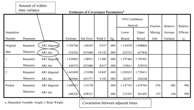
Interpretation of Output 13.3 (continued) The final table shows results for the Covariance Parameters. Again, all imputations are reported, but we only present the first 2 here. Again, information about missing data and increase in variance and efficiency following the imputation are presented. AR1 diagonal indicates the amount of within-time  variance, which is significant for all imputations.

AR1 rho indicates the covariation between adjacent time periods, which again is sizable and significant. Also, the imputation particularly increases covariation between time periods, which makes sense because times 3 and 4 were no longer missing for a number of people.

Example of How to Write About Output 13.3

Results

Eating disordered participants’ reported weight changes, predicted by level of binging at each of the four assessment times, reported mood at each of the four assessment times, level of reported preoccupation with one’s body at each assessment time, and assessment time were investigated using a Mixed Model analysis of the imputed data. An autoregressive covariance structure was selected, given the likelihood that variables would be more highly correlated at adjacent times than across more distant time points. There was a significant effect of time on weight, F (3, 200.188)= 21.58, p <.001 for original data; Fs for imputations (numerator df 3; denominator df from 226.101-228.488) ranged from 15.08-25.775, p <.001. Moreover, the model predicting weight from binging, mood, and preoccupation about body predicted significant differences between each of the first three measurements of weight and weight at the final assessment (pooled ts (dfs ranged from 220.52-312.73 for different contrasts and imputations) were -6.92, p <.001; -2.95, p=.003; -2.06, p=.041 for differences between time 1 and time 3, between time 2 and time 4, and between time 3 and time 4, respectively. Inspection of the pooled means indicated that weight increased with time from M =1.63 on a 4 point scale at time 1 to 3.02 on the same scale at time 4, which was the desired outcome for this sample of primarily anorectic individuals. There was also substantial and statistically significant within-time and between-time variance (ps <.001). Relative efficiency of the 20 imputations that exceeded .98 for all pooled estimates, suggesting that the 20 imputations provided a strong estimate of population values.

Source: Leech Nancy L. (2014), IBM SPSS for Intermediate Statistics, Routledge; 5th edition;

download Datasets and Materials.