Now that we have determined that there is significant variance to explain, we will test another model with a Level 2 predictor, gender. This analysis will enable us to answer the following question:
- Does knowing a person’s gender help us in understanding his or her growth from age 8 to age 14, as measured by the distance variable?
To answer this question, we will build on the model we just created for Problem 12.1. If you have reset the Linear Mixed Models program from the previous problem, then go back to the instructions for Problem 12.1 and redo those steps now and then do the steps that follow here. If you did not reset it, you will just need to do the following:
- Select Analyze → Mixed Models → Linear.
- Retain the settings for the first window.
- Click on Continue. This will open the Linear Mixed Models window ( 12.3).
- Keep the variables as they were in 12.3, but also move Gender into the Factors: box.
- Click on Fixed to get 12.7.
- Click to change Main Effects to Factorial in the middle box, then Click on Build nested terms. Click on linear and click on the curved arrow to add it to the build terms Click on By to add the multiplication symbol to the box, then click on gender and click on the curved arrow to move it into the box. You should see linear, quadratic, gender, and linear * gender, as in Fig. 12.7. We are looking at the interaction between linear and gender, but not between quadratic and gender because linear but not quadratic significantly predicted the outcome variable in the unconditional model, so now we want to see if an interaction with gender qualifies this effect, but we don’t want too many predictors, given the small sample size.
- Click on Add to move the interaction into the Model
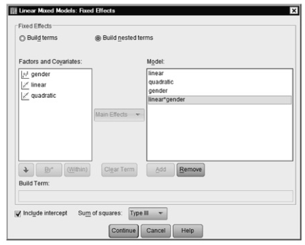
Fig. 12.7. Linear mixed models: Fixed effects.
- Click on Continue.
- Leave the settings for Random and Statistics as they are (or repeat what you did for Problem 12.1).
- Click on OK.
- Check to see if your syntax and output are like Output 12.2 below (but with additional outputs for the contrast coefficients, which we are omitting to save space).
- Unfortunately, we can’t use EM Means to calculate the means for the interaction between linear and gender because linear is a covariate instead of a factor. We can calculate this using Explore after first using Split file to calculate the means and other statistics separately for boys and girls.
- Click on Data^Split File.
- Click on Organize output by groups.
- Hit OK.
- Use Explore, as before, to calculate statistics for the dependent variable distance with factor age.
Output 12.2 Conditional Model With Gender as a Predictor
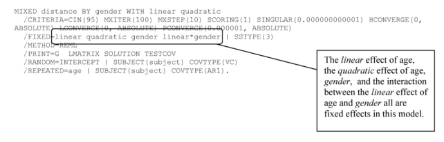
MIXED distance BY gender WITH linear quadratic
/CRITERIA=CIN(95) MXITER(IOO) MXSTEP(IO) SCORING(l) SINGULAR(0.000000000001) HCONVERGE(0 ABSOLUTE) LGONVERGE(0, ABSOLUTE) PGONVEBGE(0.000001, ABSOLUTE)
/FIXED-linear quadratic gender linear*gender I SSTYPE(3)
/METHO
/PRINT=G LMATRIX SOLUTION TESTCOV
the quadratic effect of age, gender, and the interaction between the linear effect of age and gender all are
fixed effects in this model.
Mixed Model Analysis
Interpretation of Output 12.2
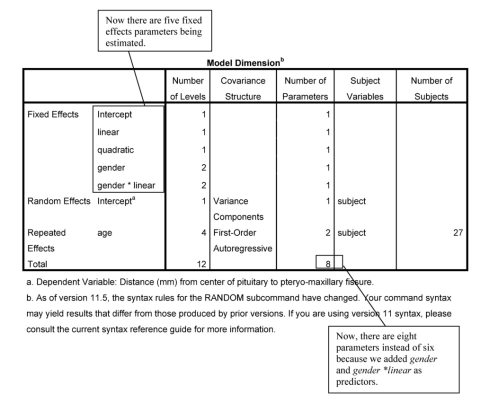
The syntax and Model Dimension tables, again, enable you to check to make sure that the program did everything as intended. Note that we have now specified 12 parameters, 4 more than we specified in the unconditional model.

Interpretation of Output 12.2 (continued) Next, you see the Information Criteria, providing goodness-of-fit data for this new model. If you compare the -2 Restricted Log Likelihood, which is a useful measure of goodness of fit, for this model (432.374) and for the unconditional model (437.43), you can see that the goodness of fit has improved by about 5. Again, smaller numbers indicate better fit. We will do a likelihood ratio shortly to see if this is a significant improvement in the model.
Fixed Effects
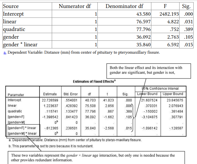
Interpretation of Output 12.2 (continued) The next table provides information about the Fixed Effects. Note that linear still is a statistically significant predictor, F(1, 76.6) = 4.82, p = .031. Now, we see that gender* linear also is a statistically significant predictor, over and above the effect of linear, F(1, 35.84) = 6.59, p = .015. However, the main effect of gender is not a statistically
significant predictor, p > .05.
We are omitting the Type III Estimable functions tables from the output reproduced here to save space, but these show you how the computer program contrasted the dummy variables.
The next table provides the parameter estimates for the fixed effects. Notice that two dummy variables were created for the gender x linear age predictor, but only one was needed because the other was redundant with it.
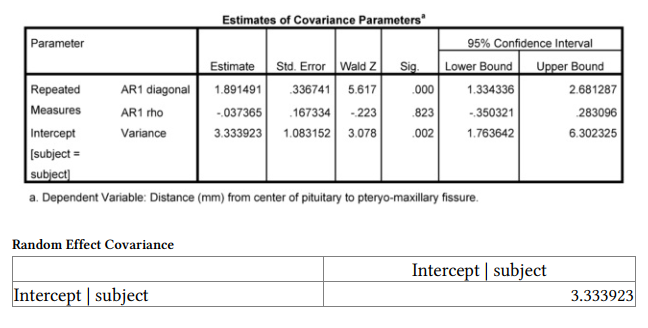
Interpretation of Output 12.2 (continued) The next table shows that the diagonal estimate (now 1.89, but 2.12 in the Level 1 model) has been reduced, suggesting that gender[1]linear explained additional variance. However, the betweenparticipants’ variability (Intercept [subject = subject]) has actually increased slightly (from 3.2 to 3.3). Moreover, the Wald statistics for both these effects suggest that there is still significant variance left to explain if we had additional predictors.
Before we show you how to write about this output, let’s calculate a chi-square to determine whether there is a significant improvement in the fit of the model because of the addition of the gender variable.
- Compute variable.
- Click on Type and Label and label this variable as Likelihood ratio sign for adding gender to linear (see Fig. 12.9).
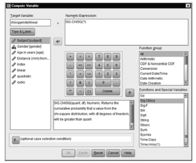
Fig.12.8.Compute variable: Type and label.
- Click on Continue. This will take you back to 12.8.
- Notice that in the Numeric expression box, CHISQ is followed by a parenthesis with a question mark. Highlight the question mark and type enter 10.37, the rounded difference between the -2 restricted log likelihoods for the conditional and the unconditional models (436.59-446.96). Next, type a comma and enter the degrees of freedom, which is the difference in number of parameters (8-6) or 2 (see Fig. 12.8). It should now look like SIG.CHISQ(10.37,2)
- Click on OK.
- If you check your Data Editor, you will see a new column on the right side, with the new variable, chiqgenderlineare. The value is .01, which means that the difference in models is significant at p =.01.Thus, adding gender and the interaction between gender and the linear effect improves the fit of the model to a statistically significant degree, as suggested by the fact that the gender x linear effect was statistically significant.
COMPUTE chisqgenderage = SIG.CHISQ(10.37,2).
VARIABLE LABELS chisqgenderage ‘Likelihood ratio sign for adding gender to age’.
EXECUTE.
Source: Leech Nancy L. (2014), IBM SPSS for Intermediate Statistics, Routledge; 5th edition;
download Datasets and Materials.
30 Mar 2023
22 Sep 2022
27 Mar 2023
15 Sep 2022
27 Mar 2023
29 Mar 2023