Problem 12.4: Conditional Individuals-Nested-in-Schools Model with Level 1 Covariate with SPSS

In Problem 12.4, we could have looked at meanses, which is a variable at the school level (Level 2) and is the average socioeconomic class for the students in a particular school. As part of this problem, we will show you how you might have calculated meanses if it were not already available. However, instead of looking at meanses in this problem, we will look at a Level 1 predictor, cses, which is students’ socioeconomic status measured as a deviation from the school’s average SES. Creating such deviation scores is called centering the data, which we will show you how to do prior to actually doing Problem 12.4. We could create a model in which we included both the Level 1 and Level 2 variables, to try to explain both within-school and betweenschool variability, but we chose not to do so.

Now that we have determined that there is significant variance to explain, we will test another model with a Level 1 predictor, cses. This analysis will enable us to answer the following question:

12.4 Does knowing a person’s socioeconomic status relative to that of the average student in his/her school (cses) help us in understanding his or her math achievement, even after the effects of differences among schools in math achievement are taken into account?

Before we do the analysis to answer this question, we will calculate a centered Level 1 variable and a Level 2 aggregate (averaged) variable to show you how to do those. Then, we will use the centered variable (which already is a part of the data set) as a Level 1 predictor in the conditional model.

• First, calculate the means for each school for SES: Click on Analyze →Descriptive Statistics → Explore.
• Highlight school and move it into the Factor List: box.
• Highlight ses and move it into the Dependent List: box.
• Under Display, click on Statistics. Your window should look like 12.16.

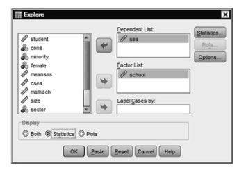
 Fig. 12.16. Explore.

• Click on OK.

Compare the mean for several schools to the values listed for meanses in your Data Editor. You will see slight rounding differences, but basically the same values for the means. Note that SES is already centered on the grand mean for all participants, so some means are negative and some are positive. Grand mean centering is another method that is commonly used in conjunction with multilevel models, especially when predictors from different levels are included in the same equation. Which mean you use in centering depends on your research question. We are not including the output for the group mean centering we are doing here in order to save space.

Now, we will center SES on each school’s mean. We’ll use meanses rather than creating a new variable based on the output we just generated.

• First, click on Transform → Compute Variable.
• Type CSES2 in the box for Target Variable.
• Click on Type and Label.
• Type in SES centered on school mean demo (see earlier example in 12.9).
• Click on Continue.
• Next, highlight and move ses into the Numeric expression box, and type – (minus sign), then type in meanses. Your window should look like Fig. 12.17.

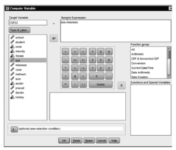
Fig.12.17.Compute variable.

• Click on

The results will appear as a new column in your data. Compare the results for a few cases to the cses variable that is already included in the data. They should be the same. We will use cses as a predictor in Problem 12.4.

We will build on the model we just created for Problem 12.3. If you have not yet reset the Linear Mixed Models program from the previous problem, you will just need to do the following:

• Select Analyze → Mixed Models → Linear.
• Retain the settings for the first window. If you reset already, then repeat the settings for 12.11.
• Click on Continue. This will open the Linear Mixed Models window ( 12.12).
• Keep the variables as they were in 12.12, but also move cses into the Covariate box to get Figure 12.18.

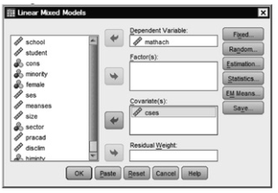
Fig.12.18.Linear mixed models.

• Click on Fixed to get 12.13.
• Click on cses, and Add it as a fixed covariate, as in 12.19.

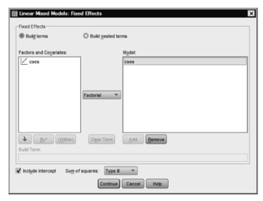
Fig. 12.19. Linear mixed models: Fixed effects.

• Click on Continue, to take you back to 12.18.
• Click on Random
• Click on r⁷ cses, and Add it as a random covariate, as in 12.20.

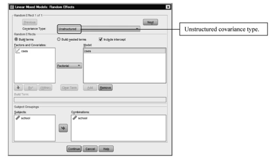
Fig. 12.20. Linear mixed models: Random effects.

• Click on Continue to take you back to 12.18.
• Click on Statistics.
• Leave the checks for Parameter estimates and Tests for covariance parameters and also check Covariances of random effects.
• Click on Continue.
• Click on OK. Compare your output with Output 12.4.

Output 12.4: Conditional Model Predicting mathach From CSES

Interpretation of Output 12.4

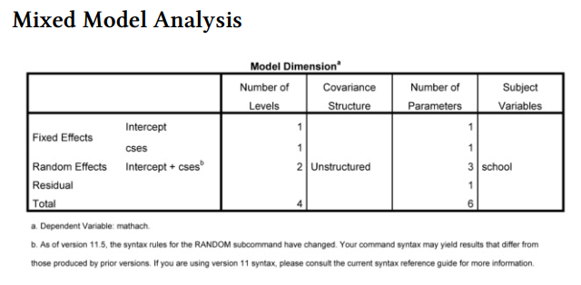
The syntax and Model Dimension tables, again, enable you to check to make sure that the program did everything as intended. Note that we have now specified six parameters, three more than we specified in the unconditional model.

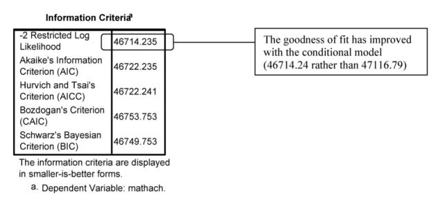
Interpretation of Output 12.4 (continued) Next, you see the Information Criteria, providing goodness-of-fit data for this new model. If you compare the -2 restricted log likelihood, which is a useful measure of goodness of fit, for this model (46714.24) and for the unconditional model (47116.80), you can see that the goodness of fit has improved by almost 403. Again, smaller numbers indicate better fit. We will again do a likelihood ratio after we go through Output 12.4, to see if this is a significant improvement in the model.

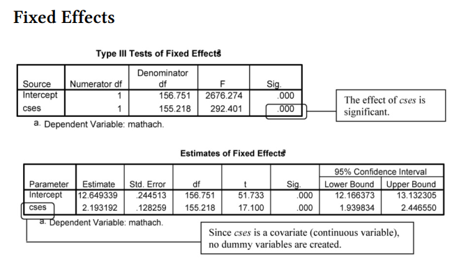
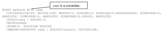
Interpretation of 12.4 continued The two previous tables provide information about the Fixed Effects. Note that cses, F(1, 155.22) = 292.4 is statistically significant at p < .001. Moreover, in the Covariance Parameters tables (next), we see that the within schools residual still is statistically significant, Wald Z = 58.65, p < .001, although, as we see by comparing this table with the one in Output 12.3, the variance component estimate has decreased from 39.15 to 36.70. This makes sense, because we are explaining some of this within-school variability by using cses as a predictor.

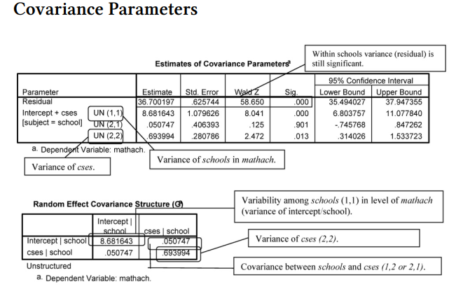
Interpretation of Output 12.4 continued The next entries in this table are less familiar and harder to interpret from the labels that are given, which is why we requested the Random Effect Covariance Structure, by checking Covariances of random effects in the Statistics menu. The line in the Estimates of Covariance Parameters table that is labeled UN (1,1) is the (unstructured) variance associated with differences between schools. As the Random Effect Covariance table indicates, the (1,1) indicates that it is the covariation of this effect with itself, or variance. In contrast to the decline in the within-schools variance component, the betweenschools variance component actually increased a negligible amount in the conditional model, from 8.61 in Output 12.3 to 8.68 in Output 12.4. The next line in the Estimates of Covariance   Parameters table, which is labeled UN (2,1), is the covariance between differences due to cses and differences between schools, as again made clearer in the Random Effect Covariance table. The final line in the Estimates of Covariance Parameters table that is labeled UN (2,2) is the variance associated with differences within schools that are due to cses.

Note that all of these effects are statistically significant except the covariance between cses and betweenschools variance. Thus, it appears that these two types of variance are relatively independent of one another.

Before we show you how to write about this output, let’s again calculate a chi­square to determine whether there is a significant improvement in the fit of the model because of the addition of the cses variable.

• First, click on Transform → Compute Variable.
• Click Reset to clear any previous settings or text.
• In the Function Group: box, highlight All.
• In the Functions and Special Variables: box, scroll down and highlight Chisq and move it into the Numeric expression: box by clicking on the up arrow to the left of the Function group: box (see Fig. 12.20).
• Notice that in the Numeric expression: box CHISQ is followed by a parenthesis with a question mark. Highlight the question mark and enter 402.56, the rounded difference between the -2 restricted log likelihoods for the conditional and the unconditional models (47116.793-46714.235). Then, type a comma and enter the degrees of freedom, which is the difference in number of parameters (6-3) or 3.
• For Target variable, type in chisqcses. Your window should look like 12.21.

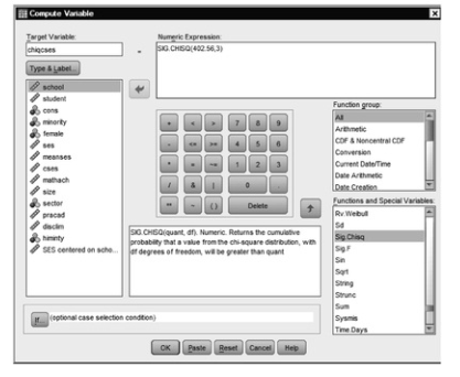
Fig. 12.21. Compute variable.

• Next, click on Type and Label and label this variable as chi square for change in school model with cses.
• Click on Continue. This will take you back to Fig. 12.21.
• Click on OK.

If you check your data, you will see a new column with the new variable. The value is .00, which means that the difference in models is significant at p < .01.

COMPUTE chiqcses=SIG.CHISQ(402.56,3).

VARIABLE LABELS chiqcses ‘chi square for change in school model with cses’.

EXECUTE.

Source: Leech Nancy L. (2014), IBM SPSS for Intermediate Statistics, Routledge; 5th edition;

download Datasets and Materials.