Measurement is the assignment of numbers or symbols to the different characteristics (values) of variables according to rules. In order to understand your variables, it is important to know their level of measurement. Depending on the level of measurement of a variable, the data can mean different things. For example, the number 2 might indicate a score of two; it might indicate that the subject was a male; or it might indicate that the subject was ranked second in the class. To help understand these differences, types or levels of variables have been identified. It is common and traditional to discuss four levels or scales of measurement, nominal, ordinal, interval, and ratio, which vary from the unordered (nominal) to the highest level (ratio).[1] [2] These four traditional terms are not the same as those used in this program, and we think that they are not always the most useful for determining what statistics to use.
SPSS uses three terms (nominal, ordinal, and scale) for the levels or types of measurement. How these correspond to the traditional terms is shown in Table 3.1. When you name and label variables with this program, you have the opportunity to select one of these three types of measurement, as was demonstrated in Chapter 2 (see Fig 2.9). An appropriate choice indicates that you understand your data and may help guide your selection of statistics.
Table 3.1. Comparison of Traditional, SPSS, and Our Measurement Terms
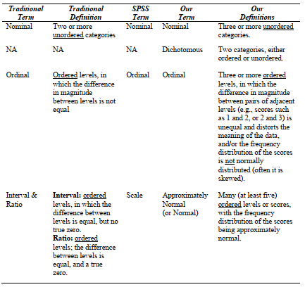
We believe that the terms nominal, dichotomous, ordinal, and approximately normal (for normally distributed) are usually more useful than the traditional or SPSS measurement terms for the selection and interpretation of statistics. In part, this is because statisticians disagree about the usefulness of the traditional levels of measurement in determining appropriate selection of statistics. Furthermore, our experience is that the traditional terms are frequently misunderstood and applied inappropriately by students. The main problem with the SPSS terms is that the term scale is not commonly used as a measurement level, and it has other meanings (see footnote 2) that make its use here confusing. Hopefully, our terms are clear and useful.
Table 3.1 compares the three sets of terms and provides a summary description of our definitions of them. Professors differ in the terminology they prefer and on how much importance to place on levels or scales of measurement, so you see all of these terms and others mentioned in textbooks and articles.
Nominal Variables
This is the most basic or lowest level of measurement, in which the numerals assigned to each category stand for the name of the category, but they have no implied order or value. For example, in the HSB study, the values for the religion variable are 1= protestant, 2 =catholic, 3 = not religious. This does not mean that two protestants equal one catholic or any of the typical mathematical uses of the numerals. The same reasoning applies to many other true nominal variables, such as ethnic group, type of disability, or section number in a class schedule. In each of these cases, the categories are distinct and nonoverlapping, but not ordered. Each category or group in the modified HSB variable ethnicity is different from every other but there is no order to the categories. Thus, the categories could be numbered 1 for Asian American, 2 for Latino American, 3 for African American, and 4 for European American or the reverse or any combination of assigning one number to each category.
What this implies is that you must not treat the numbers used for identifying nominal categories as if they were numbers that could be used in a formula, added together, subtracted from one another, or used to compute an average. Average ethnic group makes no sense. However, if you ask SPSS to compute the average ethnic group, it will do so and give you meaningless information. The important aspect of nominal measurement is to have clearly defined, nonoverlapping, or mutually exclusive categories that can be coded reliably by observers or by self-report.
Using nominal measurement does dramatically reduce the statistics that can be used with your data, but it does not altogether eliminate the possible use of statistics to summarize your data and make inferences. Therefore, even when the data are unordered or nominal categories, your research may benefit from the use of appropriate statistics. Later we discuss the types of statistics, both descriptive and inferential, that are appropriate for nominal data.
Other terms for nominal variables. Unfortunately, the literature is full of similar but not identical terms to describe the measurement aspects of variables. Categorical, qualitative, and discrete are terms sometimes used interchangeably with nominal, but we think that nominal is better because it is possible to have ordered, discrete categories (e.g., low, medium, and high IQ, which we and other researchers would consider an ordinal variable). “Qualitative” is also used to discuss a different approach to doing research, with important differences in philosophy, assumptions, and methods of conducting research.
Dichotomous Variables
Dichotomous variables always have only two levels or categories. In some cases, they may have an implied order (e.g., math grades in high school are coded 0 for less than an A or B average and 1 for mostly A or B). Other dichotomous variables do not have any order to the categories (e.g., male or female). For many purposes, it is best to use the same statistics for dichotomous and nominal variables. However, a statistic such as the mean or average, which would be meaningless for a three or more category nominal variable (e.g., ethnicity), does have meaning when there are only two categories, and when coded as dummy variables (0, 1) is especially easily interpretable. For example, in the HSB data, the average gender is .55 (with males = 0 and females = 1). This means that 55% of the participants were females, the higher code. Furthermore, we see with multiple regression that dichotomous variables, usually coded as dummy variables, can be used as independent variables along with other variables that are normally distributed.
Other terms for dichotomous variables. In the Variable View (e.g., see Fig 2.11), we label dichotomous variables “nominal,” and this is common in textbooks. However, please remember that dichotomous variables are really a special case and for some purposes they can be treated as if they were normal or scale. Dichotomous data have two discrete categories and are sometimes called discrete variables or categorical variables or dummy variables.
Ordinal Variables
In ordinal measurement, there are not only mutually exclusive categories as in nominal scales, but the categories are ordered from low to high, such that ranks could be assigned (e.g., 1st, 2nd, 3rd). Thus in an ordinal scale one knows which participant is highest or most preferred on a dimension, but the intervals between the various categories are not equal. Our definition of ordinal focuses on whether the frequency counts for each category or value are distributed like the bell-shaped, normal curve with more responses in the middle categories and fewer in the lowest and highest categories. If not approximately normal, we would call the variable ordinal. Ordered variables with only a few categories (say 2-4) would also be called ordinal. As indicated in Table 3.1, however, the traditional definition of ordinal focuses on whether the differences between pairs of levels are equal. This can be important, for example, if one will be creating summed or averaged scores (as in subscales of a questionnaire that involve aggregating a set of questionnaire items). If differences between levels are meaningfully unequal, then averaging a score of 5 (e.g., indicating the participants’ age is 65+) and a score of 2 (e.g., indicating that the participants’ age is 20-25) may not make sense. Averaging the ranks of the scores may be more meaningful if it is clear that they are ordered but that the differences between adjacent scores differ across levels of the variable. However, sometimes even if the differences between levels are not literally equal (e.g., the difference between a level indicating infancy and a level indicating preschool is not equal in years to the difference between a level of “young adulthood” and “older adulthood”), it may be reasonable to treat the levels as interval level data if the levels comprise the most meaningful distinctions and data are normally distributed.
Other terms for ordinal variables. Some authors use the term ranks interchangeably with ordinal. However, most analyses that are designed for use with ordinal data (nonparametric tests) rank the data as a part of the procedure, assuming that the data you are entering are not already ranked. Moreover, the process of ranking changes the distribution of data such that it can be used in many analyses usually requiring normally distributed data. Ordinal data are often categorical (e.g., good, better, best are three ordered categories) so ordinal is sometimes used to include both nominal and ordinal data. The categories may be discrete (e.g., number of children in a family is a discrete number; e.g., 1 or 2, etc.; it does not make sense to have a number of children in between 1 and 2.).
Approximately Normal (or Scale) Variables
Approximately normally distributed variables not only have levels or scores that are ordered from low to high, but also, as stated in Table 3.1, the frequencies of the scores are approximately normally distributed. That is, most scores are somewhere in the middle with similar smaller numbers of low and high scores. Thus a Likert scale, such as strongly agree to strongly disagree, would be considered normal if the frequency distribution was approximately normal. We think normality, because it is an assumption of many statistics, should be the focus of this highest level of measurement. Many normal variables are continuous (i.e., they have an infinite number of possible values within some range). If not continuous, we suggest that there be at least five ordered values or levels and that they have an implicit, underlying continuous nature. For example, a 5-point Likert scale has only five response categories but, in theory, a person’s rating could fall anywhere between 1 and 5 (e.g., halfway between 3 and 4).
Other terms for approximately normal variables. Continuous, dimensional, and quantitative are some terms that you will see in the literature for variables that vary from low to high, and are assumed to be normally distributed. SPSS Statistics uses scale, as previously noted. Traditional measurement terminology uses the terms interval and ratio. Because they are common in the literature and overlapping with the SPSS term scale, we describe them briefly. Interval variables have ordered categories that are equally spaced (i.e., have equal intervals between them). Most physical measurements (e.g., length, weight, temperature, etc.) have equal intervals between them. Many physical measurements (e.g., length and weight) in fact not only have equal intervals between the levels or scores, but also a true zero, which means, in the previous examples, no length or no weight. Such variables are called ratio variables. Almost all psychological scales do not have a true zero and thus even if they are very well constructed equal interval scales, it is not possible to say that zero means that one has no intelligence or no extroversion or no attitude of a certain type. However, the differences between interval and ratio scales are not important for us because we can do all of the types of statistics that we have available with interval data. SPSS Statistics terminology supports this nondistinction by using the term scale for both interval and ratio data. An assumption of most parametric statistics is that the variables be approximately normally distributed, not whether they have equal intervals between levels.
Labeling Levels of Measurement in SPSS Statistics
When you label variables with this program, the Measure column (see Fig. 2.12) provides only three choices: nominal, ordinal, or scale. How do you decide which one to use?
Labeling variables as nominal. If the variable has only two levels (e.g., Yes or No, Pass or Fail), most researchers and we would label it nominal in the SPSS Statistics variable view because that is traditional and it is often best to use the same statistics with dichotomous variables that you would with a nominal variable. As mentioned earlier, there are times when dichotomous variables can be treated as if they were ordinal; however, as long as you use numbers to code them, SPSS will still allow you to use them in such analyses. If there are three or more categories or values, you need to determine whether the categories are ordered (vary from low to high) or not. If the categories are just different names and not ordered, label the variable as nominal in the variable view. Especially if there are more than two categories, this distinction between nominal and ordered variables makes a lot of difference in choosing and interpreting appropriate statistics.
Labeling variables as ordinal. If the categories or values of a variable vary from low to high (i.e., are ordered), and there are only three or four such values (e.g., good, better, best, or strongly disagree, disagree, agree, strongly agree), we recommend that you initially label the variable ordinal. Also, even if there are five or more ordered levels or values of a variable, if you suspect that the frequency distribution of the variable is substantially non-normal, label the variable ordinal. That is, if you do not think that the distribution is approximately symmetrical and that most of the participants had scores somewhere in the middle of the distribution, call the variable ordinal. If most of the participants are thought to be either quite high or low or you suspect that the distribution will be some shape other than bell-shaped, label the variable ordinal.
Labeling variables as scale. If the variable has five or more ordered categories or values and you have no reason to suspect that the distribution is non-normal, label the variable scale in the variable view measure column. If the variable is essentially continuous (e.g., is measured to one or more decimal places or is the average of several items), it is likely to be at least approximately normally distributed, so call it scale. As you will see in Chapter 4, we recommend that you check the skewness of your variables with five or more ordered levels and then adjust what you initially called a variable’s measurement, if necessary. That is, you might want to change it from ordinal to scale if it turns out to be approximately normal or change from scale to ordinal[3] if it turns out to be too skewed.
Why We Prefer Our Four Levels of Measurement: A Review
As shown in Table 3.1 and Table 3.2, we distinguish between four levels of measurement: nominal, dichotomous, ordinal, and normal. Even though you can’t label variables as dichotomous or normal in the SPSS Statistics variable view, we think that these four levels are conceptually and practically useful. Remember that because dichotomous variables form a special case, they can be used and interpreted much like normally distributed variables, which is why we think it is good to distinguish between nominal and dichotomous even though this program does not.
Likewise, we think that normally distributed or normal is a better label than the term scale because the latter could easily be confused with other uses of the term scale (see footnote 2) and because whether or not the variable is approximately normally distributed is what, for us, distinguishes it from an ordinal variable. Furthermore, what is important for most of the inferential statistics (e.g., t test) that you will compute with SPSS is the assumption that the dependent variable must be at least approximately normally distributed.
Table 3.2. Characteristics and Examples of Our Four Levels of Measurement
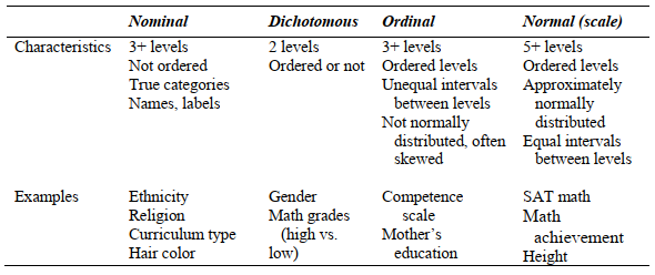
Remember that in SPSS, there are only three measurement types or levels, and you are the one who determines if the variable is called nominal, ordinal, or scale (see Fig. 2.9 again). We called dichotomous variables nominal and we have labeled approximately normal variables as scale in our hsbdata file.
[1] In this chapter, we do not phrase the creation of the outputs as “problems” for you to answer. However, we describe with bullets and arrows (as we did in Chapter 2) how to create the figures shown in this chapter. You may want to use the program to see how to create these figures and tables.
[2] Unfortunately, the terms “level” and “scale” are used several ways in research. Levels refer to the categories or values of a variable (e.g., male or female or 1, 2, or 3); level can also refer to the three or four different types of measurement (nominal, ordinal, etc.). These several types of measurement have also been called “scales of measurement,” but SPSS uses scale specifically for the highest type or level of measurement. Other researchers use scale to describe questionnaire items that are rated from strongly disagree to strongly agree (Likert scale) and for the sum of such items (summated scale). We wish there weren’t so many uses of these terms; the best we can do is try to be clear about our usage.
[3] Another alternative would be to transform the variable to normalize the distribution.
Source: Morgan George A, Leech Nancy L., Gloeckner Gene W., Barrett Karen C.
(2012), IBM SPSS for Introductory Statistics: Use and Interpretation, Routledge; 5th edition; download Datasets and Materials.
I enjoy the efforts you have put in this, regards for all the great content.