Problem 4.1: Descriptive Statistics for the Ordinal and Scale Variables with SPSS

In this problem, we use all of the HSB variables that we initially labeled as ordinal or scale in the Variable View. With those types of variables, it is important to see if the means make sense (are they close to what you expected?), to examine the dispersion/spread of the data, and to check the shape of the distribution (i.e., skewness value).

4.1. Examine the data to get a good understanding of the central tendency, variability, range of scores, and the shape of the distribution for each of the ordinal and scale variables. Which variables are normally distributed?

This problem includes descriptive statistics and ways to examine your data to see if the variables are approximately normally distributed, an assumption of most of the parametric inferential statistics that we use. Remember that skewness is an important statistic for understanding whether a variable is normally distributed; it is an index that helps determine how much a variable’s distribution deviates from the distribution of the normal curve. Skewness refers to the lack of symmetry in a frequency distribution. Distributions with a long “tail” to the right have a positive skew and those with a long tail on the left have a negative skew. If a frequency distribution of a variable has a large (plus or minus) skewness, that variable is said to deviate from normality. In this assignment, we examine this assumption for several key variables. However, some of the parametric inferential statistics that we use later in the book are robust or quite insensitive to violations of normality. Thus, we assume that it is okay to use parametric statistics to answer most of our research questions as long as the variables are not extremely skewed.

We answer Problem 4.1 by using the Descriptives command, which makes a compact, space­efficient output. You could instead run Frequencies because you can get the same statistics with that command. We use the Frequencies command later in the chapter. We use the Descriptives command to compute the basic descriptive statistics for all of the variables that we initially labeled ordinal or scale. We will not include the nominal variables (ethnicity and religion) or gender, algebra1, algebra2, geometry, trigonometry, calculus, and math grades, which are dichotomous variables but are labeled nominal here. We use them in a later problem.

4.1a. First, we will compute Descriptives for the ordinal variables. Use these steps:

• Select Analyze → Descriptive Statistics → Descriptives…
  

After selecting Descriptives, you will be ready to compute the mean, standard deviation, skewness, minimum, and maximum for all participants or cases on all the variables that we initially called ordinal under Measure in the Variable View of the Data Editor.

• While holding down the control key (i.e., the key marked “Ctrl”), click on all of the variables in the left box that we called ordinal so that they are highlighted.. These include father’s education, mother’s education, grades in h.s., and all the “item” variables (item 01 through item 11 reversed). Note that each of these variables has the symbol , which indicates that it was called ordinal in the variable view.
• Click on the arrow button pointing right to produce Fig. 4.1.
• Be sure that all of the requested variables have moved out of the left window.

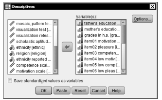
Fig. 4.1. Descriptives.

• Click on The Descriptives: Options window (Fig. 4.2) will open.
• Be sure that Mean has a check next to it.
• Under Dispersion, select Deviation, Variance, Range, Minimum, and Maximum so that each has a check.
• Under Distribution, check Your window should look like Fig.4.2

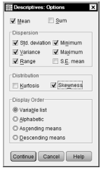
Fig. 4.2. Descriptives: Options.

• Click on Continue to get back to Fig. 4.1.
• Click on OK to produce Output 4.1a.

4.1b. Next, we compute Descriptives for the variables that were labeled scale in the Data Editor.

Note that these variables have the symbol  next to them.

• Click on Reset in Fig 4.1 to move the ordinal variables back to the left. This also deletes what we chose under Options.
• Highlight math achievement, mosaic pattern test, visualization test, visualization retest, scholastic aptitude test – math, competence scale, and motivation scale and move them to the Variables
• Click on Options and check the same descriptive statistics as you did in Fig. 4.2.

Compare your syntax output to Outputs 4.1a and 4.1b. If they look the same, you have done the steps correctly. If the syntax is not showing in your output, consult Appendix A to see how to set your computer so that the syntax is displayed.

Source: Morgan George A, Leech Nancy L., Gloeckner Gene W., Barrett Karen C.

(2012), IBM SPSS for Introductory Statistics: Use and Interpretation, Routledge; 5th edition; download Datasets and Materials.