Problem 4.2: Boxplots for One Variable and for Multiple Variables with SPSS

In addition to numerical methods for understanding your data, there are several graphic methods. In Chapter 3, we demonstrated the use of histograms and also frequency polygons (line graphs) to roughly assess normality. The trouble is that visual inspection of histograms can be deceiving because some approximately normal distributions don’t look very much like a normal curve. Thus, we don’t find the superimposed normal curve line on histograms very useful.

In this problem, we use Boxplots to examine some HSB variables. Boxplots are a method of graphically representing ordinal and scale data. They can be made with many different combinations of variables and groups. Using boxplots for one, two, or more variables or groups in the same plot can be useful in helping you understand your data.

4.2a. Create a boxplot for math achievement test.

There are several commands that will compute boxplots; we show one way here. To create a boxplot, follow these steps:

• Select Graphs→ Legacy Dialogs → Boxplot … The Boxplot window should appear.
• Select Simple and Summaries of separate variables. Your window should look like Fig. 4.3.
• Click on The Define Simple Boxplot: Summaries of Separate Variables window will appear.

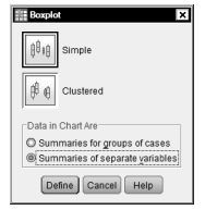
 Fig. 4.3. Boxplot.

• Highlight the variable that you are interested in (in this case, it is math achievement test). Click on the arrow to move it into the Boxes Represent When you finish, the dialog box should look like Fig. 4.4.
• Click on OK

 Fig. 4.4. Define simple boxplot: Summaries of separate variables

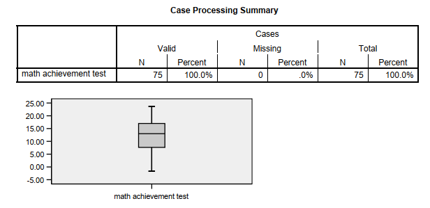
Output 4.2a: Boxplot of Math Achievement Test

EXAMINE VARIABLES=mathach /COMPARE VARIABLE/PLOT=BOXPLOT/STATISTICS=NONE/NOTOTAL /MISSING=LISTWISE .

Explore

4.2b. Compare the boxplots of competence and motivation to each other.

To create more than one boxplot on the same graph, follow these commands:

• Select Graphs → Legacy Dialogs → Boxplot … The Boxplot window should appear (see Fig. 4.3).
• Select Simple and Summaries of separate variables. Your window should again look like Fig. 4.3.
• Click on Define. The Define Simple Boxplot: Summaries of Separate Variables window will appear.
• Click on Reset.
• While holding down the control key (i.e., “Ctrl”) highlight both of the variables that you are interested in (in this case they would be competence and motivation). Click on the arrow to move them into the Boxes Represent
• Click on OK.

Output 4.2b: Boxplots of Competence and Motivation Scales

EXAMINE VARIABLES=competence motivation /COMPARE VARIABLE/PLOT=BOXPLOT

/STATISTICS=NONE/NOTOTAL

/MISSING=LISTWISE .

Explore

Notice that there are four outliers for competence and one for motivation in these boxplots. The numbers refer to which participant (line number) they represent, and the location of the dot indicates the score. So, participants 5 and 6 both scored 1 on the competence scale.

Interpretation of Outputs 4.2a and 4.2b

Outputs 4.2a and 4.2b include a Case Processing Summary table and boxplots. The Valid N, Missing cases, and Total cases are shown in the case processing summary table. In Output 4.2a, for math achievement, the valid N is 75, and there are no missing cases. The plot in Output 4.2a includes only one boxplot for our requested variable of math achievement. Each “box” represents the middle 50% of the cases and the “whiskers” at the top and bottom of the box indicate the “expected” top and bottom 25%. If there were outliers there would be “O”s and if there were really extreme scores they would be shown with asterisks, above or below the end of the whiskers. Notice that there are not any Os or *s in the boxplot in Output 4.2a.

The Case Processing table for Output 4.2b indicates that there are 71 valid cases, with 4 cases having missing data on at least one variable. The syntax indicated that this analysis involves “listwise” deletion, meaning that if a case is missing either variable, it will be omitted from boxplots for both variables. Each of the requested variables is listed separately in the case processing summary table. For the boxplot, you can see there are two separate boxplots. As indicated by the Os at the bottom of the whiskers, the boxplot for competence shows there are three outliers, and the boxplot for motivation indicates there is one outlier.

Using your output to check your data for errors. If there are Os or asterisks, then you need to check the raw data or score sheet to be sure there was not an error. The numbers next to the Os indicate the line number in the data editor next to the data of participants who have these scores. This can be helpful when you want to check to see if these are errors or if they are the actual scores of the subject. We decided not to create an identification variable because we could just use the numbers automatically assigned to each case. You can, however, make a variable that numbers each subject in some way that you find useful. Having such a variable may be helpful if you want to indicate some characteristics about participants using subject number, if you want to keep track of missing participants by skipping their ID numbers, or if you want to select certain cases by ID number for some analyses. If you wish to label outliers using such an ID number, which you have entered as a variable, you must indicate that variable in the dialog box in Fig. 4.4 where it says Label Cases by.

Using the output to check your data for assumptions. Boxplots can be useful for identifying variables with extreme scores, which can make the distribution skewed (i.e., non-normal). Also, if there are few outliers, if the whiskers are approximately the same length, and if the line in the box is approximately in the middle of the box, then you can assume that the variable is approximately normally distributed. Thus, math achievement (Output 4.2a) is near normal, motivation (4.2b) is approximately normal, but competence (4.2b) is quite skewed.

Source: Morgan George A, Leech Nancy L., Gloeckner Gene W., Barrett Karen C.

(2012), IBM SPSS for Introductory Statistics: Use and Interpretation, Routledge; 5th edition; download Datasets and Materials.