Problem 8.3: Discriminant Analysis with SPSS

Discriminant analysis is appropriate when you want to predict which group participants will be in (in this example, who took algebra 2). The procedure produces a discriminant function (or for more than two groups, a set of discriminant functions) based on linear combinations of the predictor variables that provide the best overall discrimination among the groups. The grouping or dependent variable can have more than two values, but this will increase the complexity of the output and interpretation. The codes for the grouping variable must be integers. You need to specify their minimum and maximum values, as we will in Fig. 8.3. Cases with values outside these bounds are excluded from the analysis.

Discriminant analysis (DA) is similar to multivariate analysis of variance (MANOVA, discussed in Chapter 11), except that the independent and dependent variables are switched; thus, the conceptual basis for the study is typically different. In DA, one is trying to devise one or more predictive equations to maximally discriminate people in one group from those in another group; in MANOVA, one is trying to determine whether group members differ significantly on a set of several measures. Therefore, the assumptions for DA are similar to those for MANOVA.

• What combination of gender, parents’ education, mosaic, and visualization test best distinguishes students who take Algebra 2 from those who do not?

This is a similar question to the one that we asked in Problem 8.1, but this time we will use discriminant analysis, so the way of thinking about the problem is a little different.

You can use discriminant analysis instead of logistic regression when you have a categorical outcome or grouping variable if you have all continuous independent variables. It is best not to use dichotomous predictors for discriminant analysis, except when the dependent variable has a nearly 50-50 split as is true in this case.

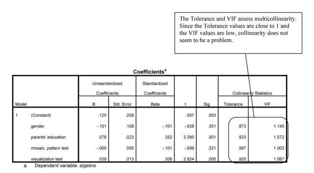
To check the condition of multicollinearity, follow these commands:

• Select Analyze → Regression → Linear.
• Highlight algebra 2 in h.s. and move it into the Dependent: box.
• Hold down the Ctrl key and highlight gender, parents’ education, mosaic,

and visualization test and move them into the Independent(s): box.

• Click on Statistics … and The Linear Regression: Statistics window will open.
• Check the box next to Collinearity diagnostics.
• Click on Continue and OK.

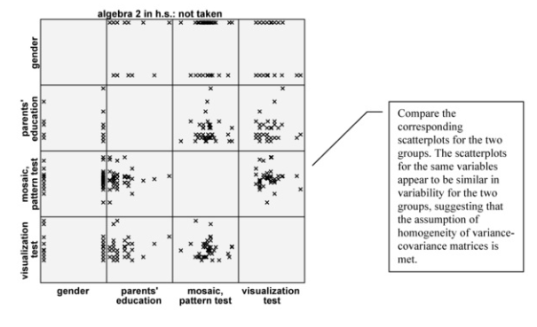
To check the assumption of linearity, we created a matrix scatterplot selecting “matrix scatter” as shown in Chapter 2, with gender, parents’ education, mosaic, and visualization test as the variables.

Next, to check the assumption of homogeneity of variance-covariance matrices across groups we created scatterplots (below) after splitting the data by the grouping variable (in this case algebra 2 in h.s.). To split the file into groups, follow these steps to use Split File.

• Select Data → Split File.
• Select Compare groups.
• Move algebra 2 in h.s. into the Groups Based on: box.
• Click on OK.

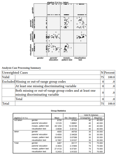
Then do two scatterplots for each level of the grouping variable.

Don’t forget to turn off the split file command before you run other analyses:

• Select Data → Split File.
• Select Analyze all cases, do not create groups.
• Click on OK.

Next, follow these steps to do the Discriminant Analysis:

• Select Analyze → Classify→ Discriminant…
• Move algebra 2 in h.s. into the Grouping Variable box (see 8.3).

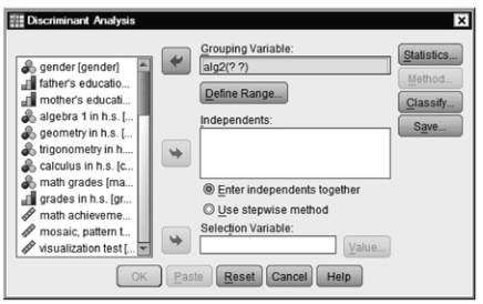
Fig. 8.3. Discriminant analysis.

• Click on Define Range and enter 0 for Minimum and 1 for Maximum (see 8.4).
• Click on Continue to return to 8.3.

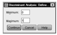
Fig.8.4.Discriminant analysis: Define range.

• Now move gender, parents’ education, mosaic, and visualization test into the Independents
• Make sure Enter independents together is selected.
• Click on Statistics.
• Select Means, Univariate ANOVAs, and Box’s M (see 8.5). Click on Continue.

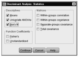
Fig.8.5.Discriminant analysis: Statistics.

• Click on Classify to get 8.6.
• Check Summary Table under Display.
• Click on Continue.

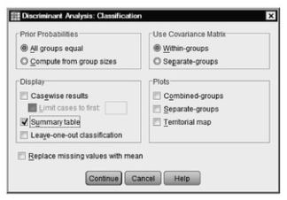
Fig. 8.6. Discriminant analysis: Classification.

• Finally, click on OK and compare your output to Output 8.3.

Output 8.3: Discriminant Analysis, Enter Independents Together

REGRESSION /MISSING LISTWISE

/STATISTICS COEFF OUTS R ANOVA COLLIN TOL

/CRITERIA=PIN(.05) POUT(.10)

/NOORIGIN

/DEPENDENT alg2

/METHOD=ENTER gender parEduc mosaic visual.

SORT CASES BY alg2.

SPLIT FILE

LAYERED BY alg2.

GRAPH

/SCATTERPLOT(MATRIX)=gender parEduc mosaic visual /MISSING=LISTWISE.

SPLIT FILE

OFF.

DISCRIMINANT

/GROUPS=alg2(0 1)

/VARIABLES=gender parEduc mosaic visual

/ANALYSIS ALL

/PRIORS EQUAL

/STATISTICS=MEAN STDDEV UNIVF BOXM TABLE

/CLASSIFY=NONMISSING POOLED.

Regression

 Graph

Interpretation of Output 8.3

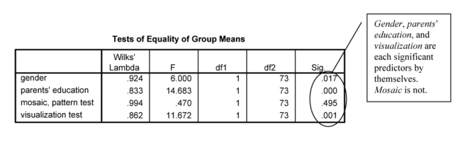
The Group Statistics table provides basic descriptive statistics for each of the independent/predictor variables for each outcome group (did not take algebra 2 and did take it) separately and for the whole sample. The Tests of Equality of Group Means table shows which independent variables are significant predictors by themselves; it shows the variables with which there is a statistically significant difference between those who took algebra 2 and those who did not. As was the case when we used logistic regression, gender, parents’ education, and visualization test are statistically significant.

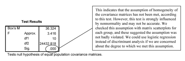
Box’s Test of Equality of Covariance Matrices

Analysis 1

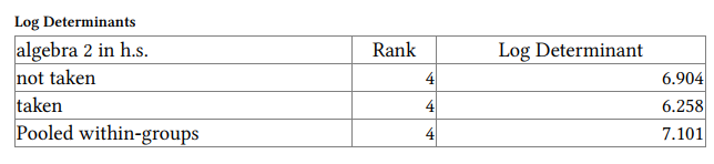
The ranks and natural logarithms of determinants printed are those of the group covariance matrices.

Summary of Canonical Discriminant Functions

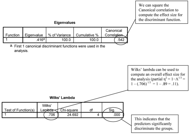
Wilks’ lambda can be used to compute an overall effect size for the analysis (partial r]² = 1-A¹³ = 1 -(.706)^1/3 = 1 – .89 = .11).

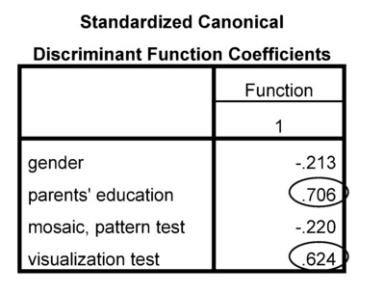
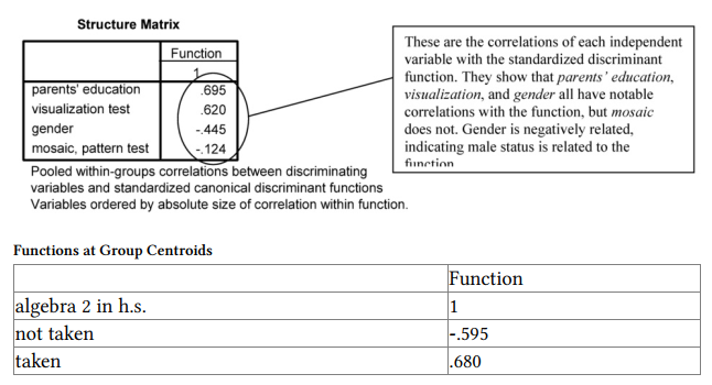
This table indicates how heavily each variable is weighted in order to maximize discrimination of groups. In this example, parents’ education and visual are weighted more than gender and mosaic.

Unstandardized canonical discriminant functions evaluated at group means

Source: Leech Nancy L. (2014), IBM SPSS for Intermediate Statistics, Routledge; 5th edition;

download Datasets and Materials.