Quantitative Longitudinal Analyses

A large number of quantitative longitudinal methods are not specific to longitu­dinal analysis, and therefore will not be developed in detail here. An example of this is regression. Nevertheless, often additional conditions have to be respected when applying these methods to longitudinal analyses – notably concerning error terms, which should be homoscedastic, and free of auto­correlation. If this condition is not respected, either the model will need to be adjusted, or procedures that are not reliant on the variance-covariance assump­tions must be used (for more details, see Bergh and Holbein, 1997).

1. Event Analysis Methods

Longitudinal analyses are often chosen because a researcher is particularly con­cerned with certain events that may affect the life of an organization. When the event itself is the object of study, the event history analysis method is used. If, however, the event is not the subject of the study, but the research seeks to dis­cern the influence of a certain event on the actual subject, the event study method would be used.

1.1. Event history analysis

Any relatively sudden qualitative change that happens to an individual or to an organization can be classed as an event. Examples of events that may occur include an individual being promoted or dismissed, or an organization experi­encing a strike or a takeover bid.

One could consider using regression for an event study. However, regres­sion entails a risk of introducing a bias into the results, or of losing information. In fact, the data that is collected possesses two characteristics that violate the assumptions underlying ‘classic’ regression (Allison, 1984). The first of these characteristics appears when data have been collected on the possible causes of an event: explanatory variables can change over the observation period. Imagine, for example, a study trying to identify how much time will pass between when a company begins exporting and when it establishes a presence abroad. Those companies that began exporting in 1980 could be used as a sam­ple, observing in each case whether they have established a presence abroad, and if so, when this occurred, along with possible explanations. For example, sales figures achieved overseas could possibly result in consolidating a com­pany’s position there. The problem we encounter here is that the explanatory variables could change radically during the study. A company that established itself overseas in 1982 could sustain a sharp increase in export sales figures because of this fact. Sales figures, from being a cause of the foreign develop­ment, then become a consequence of it.

The second characteristic of the collected data that prevents the use of clas­sical regression is known as censoring: this refers to the situation when data collection has been interrupted by the end of the study. In our example, infor­mation is gathered on the establishment of companies overseas from 1980 to the present. At the end of the studied period, certain companies will not have established themselves overseas, which poses a major problem. We do not know the value of the explanatory variables for these companies (the period between beginning to export and establishing a presence). This value is then said to be ‘censored’. The only possible solutions to such a situation could lead to serious biases: to eliminate these companies from the sample group would strongly bias it and make the results questionable; to replace the missing data with any particular value (including a maximum value – the time from 1980 to the end of the study), would minimize the real value and so once again falsify the results.

Another important concept when analyzing event history concerns the risk period (Yamaguchi, 1991). The time in which the event is not happening can generally be broken into two parts: the period in which there is a risk the event will happen, and the period in which occurrence of the event is not possible. For example, if the studied event is the dismissal of employees, the risk period corresponds to the time the studied employees have a job. When they do not have a job, they are at no risk of losing it. We can also speak in terms of a risk set to refer to those individuals who may experience the event.

Two groups of methods can be used to study transition rates: parametric and semi-parametric methods on the one hand, and non-parametric methods on the other. The first are used to develop hypotheses of specific distribution of time (generally of exponential distributions, such as Weibull or Gompertz), and aim to estimate the effects of explanatory variables on the hazard rate. Non­parametric methods, however, do not generate any hypotheses on the distribu­tion of time, nor do they consider relationships between the hazard rate and the explanatory variables. Instead, they are used to assess the hazard rate specific to a group, formed according to a nominal explanatory variable that does not change over time.

1.2. Event study

The name ‘event study’ can be misleading: it does not refer to studying a par­ticular event, but rather its impact on the object of the research. Event study methods measure how a dependent variable will evolve in the light of the occurrence of a particular event. The evolution of this variable is therefore mea­sured both before and after the occurrence of the event. Through an OLS regres­sion, the researcher tries to estimate what the value of the dependent variable would have been on the date the event occurred, had that event not taken place. The difference between the calculated value and the real value is called abnor­mal return, and it is considered to correspond to the effect of the event. This abnormal return is generally standardized by dividing it by its standard devi­ation. However, it can happen that the effect of the event takes place on a dif­ferent date (before the event, if it was anticipated, or after it, if the event had a delayed impact). The impact might also be diluted over a somewhat longer period, called an event window – in which case we can calculate the sum of the differences between the estimated values and those observed in the event win­dow. If the aggregate difference is not zero, the following test will be used to verify whether it is significant:

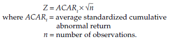
McWilliams and Siegel (1997) emphasize the precautions that must be taken with such types of analysis. First, the sample should be reasonably large, as the test statistics used are based on normality assumptions. Moreover, OLS regres­sions are very sensitive to outliers, which should therefore be identified, espe­cially if the sample is small. Another major difficulty concerns the length of the event window. It should be as short as possible, to exclude disruptive elements, external to the study, while still remaining long enough to capture the impact of the event. Finally, the abnormal returns should be justified theoretically.

2. Sequence Methods

Sequence methods are used to study processes. One type of research that can be conducted using these methods consists in recognizing and comparing sequences. We could, for example, establish a list of the different positions held by CEOs (chief executive officers) of large companies over their careers, as well as the amount of time spent at each post. The sequences formed in this way could then be compared, and typical career paths could be determined.

Another type of research could aim at determining the order of occurrence of the different stages of a process. For example, the classic decision models indicate that in making decisions we move through phases of analyzing the problem, researching information, evaluating the consequences and making a choice. But in reality, a single decision can involve returning to these different steps many times over, and it would be difficult to determine the order in which these stages occur ‘on average’.

2.1. Comparing sequences

Sequence comparison methods have to be chosen according to the type of data available. We can distinguish sequences according to the possibility of the recurrence or non-recurrence of the events they are composed of, and accord­ing to the necessity of knowing or not knowing the distance between these events. The distance between events can be assessed by averaging the tempo­ral distance between them across all cases, or on the basis of a direct categori­cal resemblance, or by considering transition rates (Abbott, 1990).

The simplest case is a sequence in which every event is observed once and only once (non-recurrent sequence). In this case, two sequences can be compared using a simple correlation coefficient. Each sequence is arranged in order of occurrence of the events it is composed of, and the events are numbered accord­ing to their order of appearance. The sequences are then compared two by two, using a rank correlation coefficient. The higher the coefficient (approaching 1) the more similar the sequences are. A typical sequence can then be established: the sequence from which the others differ least. A typology of possible sequences could also be established, using a typological analysis (such as hierarchical or non-hierarchical classification, or multidimensional analysis of similarities). This procedure does not require measuring the distances between events.

The most frequently used measure of correlation is the Spearman rank cor­relation coefficient. It is calculated in the following manner:

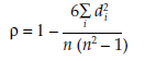
where

d_i = distance between the two classifications of event i

n = number of classified events.

This coefficient assumes that the ranks are equidistant – in other words, that the distance between ranks 3 and 4 is equal to the distance between ranks 15 and 16, for example. For cases in which it seems that this hypothesis is not appropriate, we can use the Kendall’s tau, which is calculated as follows:

where

n_a = number of agreements between two classifications (any pair of objects classed in the same rank order both times)

n_d = number of discrepancies between two classifications (any pair of objects classed in different rank-order)

N = number of possible pairs.

Third, if the classifications reveal any tied events, an index such as Goodman and Kruskal’s gamma should be used, with the following formula:

In the case of recurring sequences, the most popular approach is to use a Markov chain, or process, which postulates that the probability of an event occurring depends entirely on its immediate predecessor. A Markov chain is defined with the conditional probabilities that make up the matrix of transitions. This matrix groups estimations based on observed proportions (the percentage of times an event is followed by another – or by itself, on the matrix diagonal).

Another possibility for recurring sequences consists of a group of tech­niques called optimal matching. The optimal matching algorithm between two sequences begins with the first sequence and calculates the number of addi­tions or suppressions necessary to produce the second sequence (Abbott and Forrest, 1986). The necessary transitions are weighted according to the distance between the events. We then obtain a matrix of distance between sequences, which can be used in sequence comparisons.

2.2. Determining order of occurrence

Other types of research can be used to determine the order of occurrence of events. In this case the researcher wants to identify a general pattern from a mass of events. One of these methods was proposed by Pelz (1985), who applied it to analyzing innovation processes. The method is based on Goodman and Kruskel’s gamma, and allows the order of observed events to be estab­lished, as well as defining to what extent these events overlap.

The calculation method comprises the following steps:

• The number P of times that event A happens before event B is counted.
• The number Q of times that event B happens before event A is counted.
• The gamma is calculated for each pair of events as follows:

γ is between +1 and -1.

• Repeating the process for each pair of events enables a squared gamma matrix to be established, with a number of lines equal to the total number of events.

From this gamma matrix the researcher can calculate a time sequence score, which determines in which order the events took place, and a separation score, which indicates whether the events are separated from one another or if they overlap.

The time sequence score is obtained by calculating the mean from the columns of gamma values. In this way, a score ranging from + 1 to – 1 is ascribed to each event. By reclassifying the events according to their score, in diminishing order, the events are ordered chronologically.

The separation score is obtained by calculating the mean from the columns of absolute gamma values. Each event is credited with a score of between 0 and 1. It is generally considered that an event for which the score is equal to or above 0.5 is clearly separated from those that surround it, whereas an event with a score lower than 0.5 cannot be separated from the events that surround it and therefore must be grouped with these events (Poole and Roth, 1989).

Interpretation of Pelz’s gamma, in which a high gamma indicates that two events are separate, rather than associated, is opposite to the interpretation of Goodman and Kruskal’s gamma, on which the method is based. This is because it is calculated using the two variables time and the passage of event A to an event B. A high gamma therefore, indicates that the passage from A to B is strongly associated with the passage of time. The interpretation that can be drawn is that A and B are strongly separated.

An important advantage of this method is that it is independent of the time elapsed between events: therefore it is not necessary for this information to be available. In fact, the results do not change if the interval of time between the two incidents differs. The only point that has to be observed in relation to time is chronological order.

3. Cohort Analysis

Cohorts represent groups of observations having in common the fact that they have experienced the same event within a given period of time. The event in question is frequently birth but could be any notable event. The period of this event may extend over a variable duration, often between one and ten years. But for very dramatic events it can be considerably reduced. Cohort analysis enables us to study changes in behavior or attitudes in these groups. We can observe three types of changes: changes in actual behavior, changes due to aging, or changes due to an event occurring during a particular period (Glenn, 1977). We can distinguish intra-cohort analysis, focusing on the evolution of a cohort, from intercohort analysis, in which the emphasis is on comparisons.

3.1. Intra-cohort analysis

Intra-cohort analysis consists in following a cohort through time to observe changes in the phenomenon being studied. Let us imagine that we want to study the relationship between the age of a firm and its profitability. We could select a cohort, say that of companies created between 1946 and 1950, and follow them over the course of time by recording a profitability measure once a year. This very simple study of a trend within a cohort does, however, raise several problems. First, a certain number of companies will inevitably drop out of the sample over time. It is, in fact, likely that this mortality in the sample will strongly bias the study, because the weakest companies (and therefore the least profitable) are the most likely to disappear. Another problem is that intra-cohort analyses generally use aggregated data, in which effects can counterbalance each other. For example, if half the companies record increased profits, while the other half record a decrease in their profits of equal proportions, the total effect is nullified. Methods originally developed for studying panel data can, however, be used to resolve this problem.

A third problem raised by intra-cohort studies is that our study will not enable us to ascertain the true impact of company age on profitability. Even if we observe a rise in profitability, we will not know if this is due to the age of the company or to an external event – an effect of history such as a particularly favorable economic situation. Other analyses are therefore necessary.

3.2. Inter-cohort analysis

Among the other analyses just mentioned, one method is to compare several cohorts at a given time. In our case, this could bring us to compare, for example, the profitability in 1990 of companies created at different periods. In this we are leaving the domain of longitudinal analysis, though, as such a study is typically cross-sectional. Second, this design on its own would not enable us to resolve our research question. In fact, any differences we might observe could be attributed to age, but also to a cohort effect: companies established in a certain era may have benefited from favorable economic circumstances and may continue to benefit from those favorable circumstances today.

3.3. Simultaneous analysis of different cohorts

The connection between age and profitability of companies can be established only by simultaneous intra- and inter-cohort analysis. Changes observed in the performance levels of companies could be due to three different types of effects: the effects of age (or that of aging, which is pertinent in this case), cohort effects (the fact of belonging to a particular cohort), and period effects (the time at which profitability is measured). To try to differentiate these effects, a table can be estab­lished with rows representing the cohorts and with the observation periods recorded in columns. Where it is possible to separate data into regular intervals this should always be preferred. The period between readings should also be used to delimit the cohorts. For example, if the data easily divides into ten-year intervals, ten-year cohorts are preferable – although this is not always possible, it does make for better analyses. The resulting table can be used to complete intra­cohort and inter-cohort analyses. If identical time intervals have been used for the rows and the columns (for example, ten-year intervals), the table presents the advantage that the diagonals will give the intra-cohort tendencies (Glenn, 1977).

All the same, the differences observed between the cells of the table have to be analyzed with caution. First, these differences should always be tested to see if they are statistically significant. Second, the findings may have been biased by the mortality of the sample, as we mentioned earlier. If the elements that have disappeared did not have the same distribution as those that remain, the structure of the sample will change. Finally, it is very difficult to differentiate the three possible effects (age, cohort, and period), because they are linearly dependent, which poses problems in analyses such as regression, where the explanatory variables must be independent. Here, in the case of a birth cohort, the three factors are linked by the relationship:

cohort = period – age

A final possibility consists in recording each age, each cohort, and each period as a dummy variable in a regression. However, this leads us to form the hypo­thesis that the effects do not interact: for example, that the effect of age is the same for all the cohorts and all the periods, which is usually unrealistic (Glenn, 1977).

Source: Thietart Raymond-Alain et al. (2001), Doing Management Research: A Comprehensive Guide, SAGE Publications Ltd; 1 edition.