Retail Merchandise Forecasting and Budgeting: Dollar Control

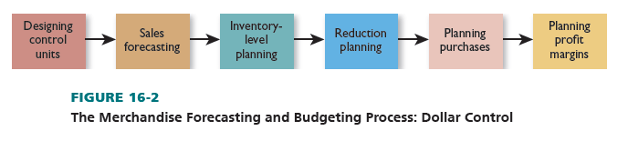
As we noted earlier, dollar control entails planning and monitoring a firm’s inventory investment over time. Figure 16-2 shows the six-step dollar control process for merchandise forecasting and budgeting. This process should be followed sequentially since a change in one stage affects all the stages after it. If a sales forecast is too low, a firm may run out of items because it does not plan to have enough merchandise during a selling season and planned purchases will also be too low.

1. Designating Control Units

Merchandise forecasting and budgeting requires the selection of control units, the merchandise categories for which data are gathered. Such classifications must be narrow enough to isolate opportunities and problems with specific merchandise lines. A retailer wishing to control goods within departments must record data on dollar allotments separately for each category.

Knowing that total markdowns in a department are 20 percent above last year’s level is less valuable than knowing the specific merchandise lines in which large markdowns are being taken. A retailer can broaden its control system by combining categories that comprise a department. However, a broad category cannot be broken down into components.

It is helpful to use control units consistent with company and trade association data. Internal com­parisons are meaningful only if categories are stable. Classifications that shift over time do not permit comparisons. External comparisons are not meaningful if control units are dissimilar for a retailer and its trade associations. Control units may be based on departments, classifications in departments, price-line classifications, and standard merchandise classifications. A discussion of each follows.

The broadest practical classification for financial records is the department, which lets a retailer assess each general merchandise grouping or buyer. Even small Handy Hardware needs departmental data (tools and equipment, supplies, housewares, and so on) for buying, inventory control, and markdown decisions. For more financial data, classification merchandising can be used, with each department subdivided into further categories for related types of merchandise. In planning its tools and equipment department, Handy Hardware can keep financial records on both overall departmental performance and the results of such categories as lawn mowers/snow blowers, power tools, hand tools, and ladders.

A special form of classification merchandising uses price line classifications—sales, inven­tories, and purchases are analyzed by price category. This helps if distinct models of a product are sold at different prices to dissimilar target markets (such as Handy’s having $50 power tools for do-it-yourselfers and $135 models for contractors). Retailers with deep assortments most often use price line control.

To best contrast its data with industry averages, a firm’s merchandise categories should con­form to those cited in trade publications. The National Retail Federation devised a standard mer­chandise classification with common reporting categories for a range of retailers and products. Specific classifications are also popular for some retailers. Progressive Grocer regularly publishes data based on standard classifications for supermarkets.

Once appropriate dollar control units are set, all transactions—including sales, purchases, transfers, markdowns, and employee discounts—must be recorded under the proper classification number. Thus, if house paint is Department 25 and brushes are 25-1, all transactions must carry these designations.

2. Sales Forecasting

A retailer estimates its expected future revenues for a given period by sales forecasting. Forecasts may be companywide, departmental, and for individual merchandise classifications. Perhaps the most important step in financial merchandise planning is accurate sales forecasting, because an incorrect projection of sales throws off the entire process. That is why many retailers use state-of- the-art forecasting software. Unified Grocers has dramatically improved its inventory productivity by using such software from SAS.³

Larger retailers often forecast total and department sales by techniques such as trend analysis, time-series analysis, and multiple regression analysis. A discussion of these techniques is beyond the scope of this book. Small retailers rely more on “guesstimates,” projections based on experi­ence. Even for larger firms, sales forecasting for merchandise classifications within departments (or price lines) relies on more qualitative methods. One way to forecast sales for narrow categories is first to project sales on a company basis and then by department, and finally to break down figures judgmentally into merchandise classifications.

External factors, internal company factors, and seasonal trends must be anticipated and taken into account. Among the external factors that can affect projected sales are consumer trends, competitors’ actions, the state of the economy, the weather, and new supplier offerings. For exam­ple, Planalytics offers a patented methodology to analyze and forecast the relationship among consumer demand, store traffic, and the weather.⁴ Internal company factors that can affect future sales include additions and deletions of merchandise lines, revised promotion and credit poli­cies, changes in hours, new outlets, and store remodeling. With many retailers, seasonality must be considered in setting monthly or quarterly sales forecasts. Handy’s yearly snow blower sales should not be estimated from December sales alone.

A sales forecast can be developed by examining past trends and projecting future growth (based on external and internal factors). Table 16-7 shows a sales forecast for Handy Hardware. It is an estimate, subject to revisions. Various factors may be hard to incorporate when devising a forecast, such as merchandise shortages, consumer reactions to new products, the rate of inflation, and new government legislation. That is why a financial merchandise plan needs some flexibility.

After a yearly forecast is derived, it should be broken into quarters or months. In retailing, monthly forecasts are typical. Jewelry stores know December accounts for nearly one-quarter of annual sales, whereas drugstores know December sales are slightly better than average. Stationery stores and card stores realize that Christmas and other holiday cards generate more than 30 percent of seasonal greeting card sales, and Valentine’s Day cards are second with about 15 percent.⁵

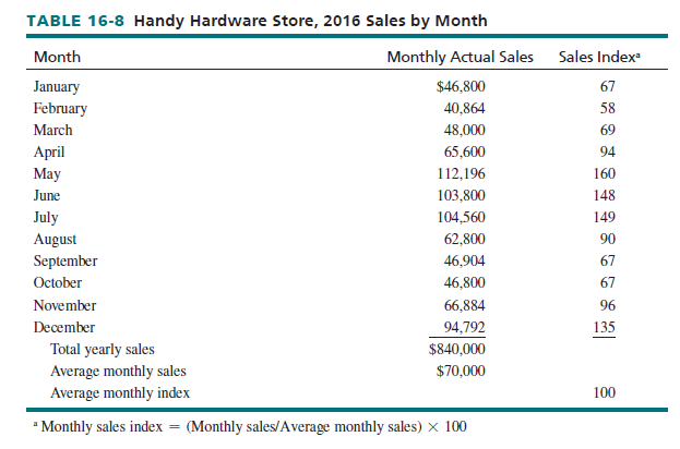
To acquire more specific estimates, a retailer could use a monthly sales index that divides each month’s actual sales by average monthly sales and multiplies the results by 100. Table 16-8 shows Handy Hardware’s 2016 actual monthly sales and monthly sales indexes. The store is seasonal, with peaks in late spring and early summer (for lawn mowers, garden sup­plies, and so on), as well as December (for lighting fixtures, snow blowers, and gifts). Average monthly 2016 sales were $70,000 ($840,000/12). Thus, the monthly sales index for January is 67[($46,800/$70,000) X 100]; other monthly indexes are computed similarly. Each monthly index shows the percentage deviation of that month’s sales from the average month. A May index of 160 means May sales are 60 percent higher than average. An October index of 67 means sales in October are 33 percent below average.

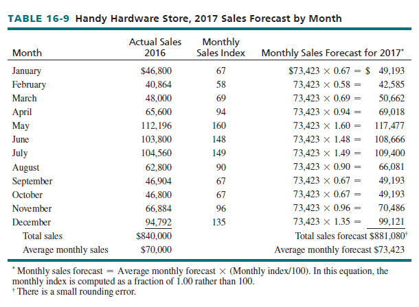
After monthly sales indexes are determined, a retailer can forecast monthly sales, based on the yearly sales forecast. Table 16-9 shows how Handy’s 2017 monthly sales can be forecast if average monthly sales are expected to be $73,423.

3. Inventory-Level Planning

At this point, a retailer plans its inventory. The level must be sufficient to meet sales expectations, allowing a margin for error. Techniques to plan inventory levels are the basic stock, percentage variation, weeks’ supply, and stock-to-sales methods.

With the basic stock method, a retailer carries more items than it expects to sell over a speci­fied period. There is a cushion if sales are more than expected, shipments are delayed, or customers want to select from a variety of items. It is best when inventory turnover is low or sales are erratic over the year. Beginning-of-month planned inventory equals planned sales plus a basic stock amount:

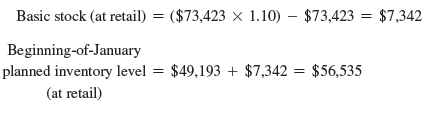
If Handy Hardware, with an average monthly 2017 forecast of $73,423, wants extra stock equal to 10 percent of its monthly forecast and expects January 2017 sales to be $49,193:

In the percentage variation method, beginning-of-month planned inventory during any month differs from planned average monthly stock by only one-half of that month’s variation from estimated average monthly sales. This method is recommended if stock turnover is more than six times a year or relatively stable, since it results in planned inventories closer to the monthly average than other techniques:

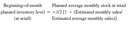
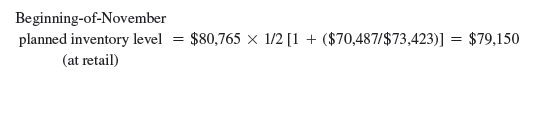
If Handy Hardware plans average monthly stock of $80,765 and November 2017 sales are expected to be 4 percent less than average monthly sales of $73,423, the store’s planned inventory level at the beginning of November 2017 would be:

Handy Hardware should not use this method due to its variable sales. If it did, Handy would plan a beginning-of-December 2017 inventory of $94,899, less than expected sales ($99,121).

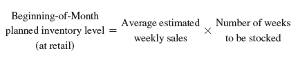
The weeks’ supply method forecasts average sales weekly, so beginning inventory equals several weeks’ expected sales. It assumes inventory is in proportion to sales. Too much merchan­dise may be stocked in peak periods and too little during slow periods:

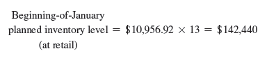
If Handy Hardware forecasts average weekly sales of $10,956.92 from January 1, 2017, through March 31, 2017, and it wants to stock 13 weeks of merchandise (based on expected turnover), beginning inventory would be $142,440:

With the stock-to-sales method, a retailer wants to maintain a specified ratio of goods on hand to sales. A ratio of 1.3 means that if Handy Hardware plans sales of $69,018 in April 2017, it should have $89,723 worth of merchandise (at retail) available during the month. Like the weeks’ supply method, this approach tends to adjust inventory more drastically than changes in sales require.

Yearly stock-to-sales ratios by retail type are provided by sources such as Industry Norms & Key Business Ratios (New York: Dun & Bradstreet) and Annual Statement Studies (Philadelphia: RMA). These sources will allow a retailer to compare its ratios with those of other firms.

4. Reduction Planning

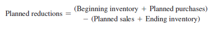
Besides forecasting sales, a firm should estimate its expected retail reductions, which represent the difference between beginning inventory plus purchases during the period and sales plus ending inventory. Planned reductions incorporate anticipated markdowns (discounts to stimulate sales), employee and other discounts (price cuts to employees, senior citizens, and others), and stock shortages (pilferage, breakage, and bookkeeping errors):

Reduction planning revolves around two key factors: estimating expected total reductions by budget period and assigning estimates monthly. The following should be considered in planning reductions: past experience, markdown data for similar retailers, changes in company policies, merchandise carryover from one budget period to another, price trends, and stock-shortage trends.

Past experience is a good starting point. The data can then be compared with the performance of similar firms—by reviewing data on markdowns, discounts, and stock shortages in trade pub­lications. A retailer with higher markdowns than those of its competitors could investigate and correct the situation by adjusting its buying practices and price levels or improve the training of sales personnel.

A retailer must consider its own procedures in reviewing reductions. Policy changes often affect the quantity and timing of markdowns. If a firm expands its assortment of seasonal and fashion merchandise, this would probably lead to a rise in markdowns.

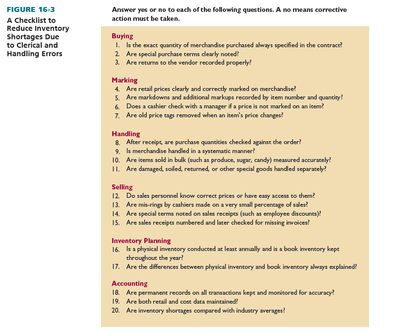
Merchandise carryover, price trends, and stock-shortage trends also affect planning. If such items as gloves and antifreeze are stocked in off seasons, markdowns are often not used to clear out inventory. Yet, the carryover of fad items merely postpones reductions. Price trends of product categories have a strong impact on reductions. Many full computer systems now sell for less than $1,000, down considerably from prior years. This means higher-priced computers must be marked down. Recent stock shortage trends (comparing prior book and physical inventory values) can be used to project future reductions due to employee, customer, and vendor theft; breakage; and bookkeeping mistakes. If a firm has stock shortages of less than 2 percent of annual sales, it is usually deemed to be doing well. Figure 16-3 shows a checklist to reduce shortages from clerical and handling errors. Suggestions for reducing shortages from theft were covered in Chapter 15.

After determining total reductions, they must be planned by month because reductions as a percentage of sales are not the same during each month. Stock shortages may be much higher during busy periods, when stores are more crowded and transactions happen more quickly.

5. Planning Purchases

The formula for calculating planned purchases for a period is:

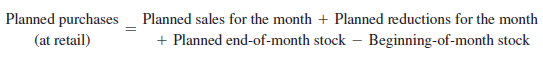
If Handy Hardware projects June 2017 sales to be $108,666 and total planned reductions to be 5 percent of sales, plans end-of-month inventory at retail to be $72,000, and has a beginning- of-month inventory at retail of $80,000, planned purchases for June are:

Planned purchases
(at retail) = +108,666 + +5,433 + +72,000 – +80,000 = +106,099

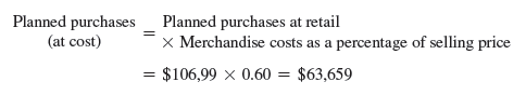
Because Handy Hardware expects 2017 merchandise costs to be about 60 percent of retail selling price, its plan is to purchase $63,659 of goods at cost in June 2017:

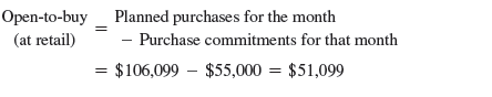
Open-to-buy is the difference between planned purchases and the purchase commitments already made by a buyer for a given period, often a month. It represents the amount the buyer has left to spend for that month and is reduced each time a purchase is made. At the beginning of a month, a firm’s planned purchases and open-to-buy are equal if no purchase commitments have been made before that month starts. Open-to-buy is recorded at cost.

At Handy Hardware, the buyer has made purchase commitments for June 2017 in the amount of $55,000 at retail. Accordingly, Handy’s open-to-buy at retail for June is $51,099:

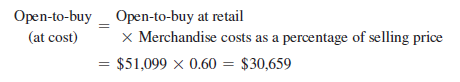
To calculate the June 2017 open-to-buy at cost, $51,099 is multiplied by Handy Hardware’s merchandise costs as a percentage of selling price:

The open-to-buy concept has two major strengths: (1) It maintains a specified relationship between inventory and planned sales, which avoids overbuying and underbuying and (2) it lets a firm adjust purchases to reflect changes in sales, markdowns, and so on. If Handy revises its June 2017 sales forecast to $120,000 (from $108,666), it automatically increases planned purchases and open-to-buy by $11,334 at retail and $6,800 at cost.

It is advisable for a retailer to keep at least a small open-to-buy figure for as long as possible— to take advantage of special deals, purchase new models when introduced, and fill in items that sell out. An open-to-buy limit sometimes must be exceeded due to underestimated demand (low sales forecasts). A retailer should not be so rigid that merchandising personnel are unable to have the discretion (employee empowerment) to purchase below-average-priced items when the open- to-buy is not really open.

6. Planning Profit Margins

In preparing a profitable merchandise budget, a retailer must consider planned net sales, retail operating expenses, profit, and retail reductions in pricing merchandise:

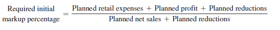
The required markup is a firmwide average. Individual items may be priced according to demand and other factors, as long as the average is met. The concept of initial markup is introduced here for continuity in the description of merchandise budgeting. A fuller discussion on markup can be found in Chapter 17.

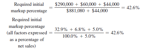
Handy has an overall 2017 sales forecast of $881,080 and expects annual expenses to be $290,000. Reductions are projected at $44,000. The total net dollar profit margin goal is $60,000 (6.8 percent of sales). Its required initial markup is 42.6 percent:

Source: Barry Berman, Joel R Evans, Patrali Chatterjee (2017), Retail Management: A Strategic Approach, Pearson; 13th edition.