Sales and Operations Planning at Red Tomato in the Supply Chain

Promotion decisions are often made by retailers without taking into account the impact on the rest of the supply chain. In this section, our goal is to show how supply chain members can col­laborate on pricing and aggregate planning (both demand and supply management) decisions to maximize supply chain profitability. Let us return to Red Tomato Tools, the gardening tools manufacturer discussed in Chapter 8. Green Thumb Gardens is a large retail chain that has signed an exclusive contract to sell all products made by Red Tomato Tools. Demand for garden tools peaks in the spring months of March and April, as gardeners prepare to begin planting. In plan­ning, the goal of both firms should be to maximize supply chain profits, because this outcome leaves them more money to share. For profit maximization to take place, Red Tomato and Green Thumb need to devise a way to collaborate and, just as important, determine a way to split the supply chain profits. Determining how these profits will be allocated to different members of the supply chain is key to successful collaboration.

Red Tomato and Green Thumb are exploring how the timing of retail promotions affects profitability. Are they in a better position if they offer the price promotion during the peak period of demand or during a low-demand period? Green Thumb’s vice president of sales favors a pro­motion during the peak period because this increases revenue by the largest amount. In contrast, Red Tomato’s vice president of manufacturing is against such a move because it increases manu­facturing costs. She favors a promotion during the low-demand season because it levels demand and lowers production costs. S&OP allows the two to collaborate and make the optimal trade-offs.

1. The Base Case

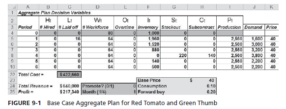
We start by considering the base case discussed in Chapter 8. Each tool has a retail price of $40. Red Tomato ships assembled tools to Green Thumb, where all inventory is held. Green Thumb has a starting inventory in January of 1,000 tools. At the beginning of January, Red Tomato has a workforce of 80 employees at its manufacturing facility in Mexico. There are 20 working days in each month, and Red Tomato workers earn the equivalent of $4 per hour. Each employee works eight hours on normal time and the rest on overtime. Because the Red Tomato operation consists mostly of hand assembly, the capacity of the production operation is determined primarily by the total labor hours worked (i.e., it is not limited by machine capacity). No employee works more than 10 hours of overtime per month. The various costs are shown in Table 9-2.

There are no limits on subcontracting, inventories, and stockouts. All stockouts are back­logged and supplied from the following month’s production. Inventory costs are incurred on the ending inventory in each month. The companies’ goal is to obtain the optimal aggregate plan that leaves at least 500 units of inventory at the end of June (i.e., no stockouts at the end of June and at least 500 units in inventory). The base demand forecast is shown in cells J5:J10 of Figure 9-1.

All figures and analysis in this chapter come from the spreadsheet Chapter8,9-examples, which uses Solver. The equivalent solutions can also be obtained without Solver using the spreadsheet Chapter8-trial-aggplan. The spreadsheet contains instructions for use and worksheets corre­sponding to Figures 9-1 to 9-5.

For the base case, we set cell E24 to 0 (no promotion) and use Solver. The optimal base case aggregate plan for Red Tomato and Green Thumb is shown in Figure 9-1 (this is the same as discussed in Chapter 8 and shown in Table 8-4).

For the base case aggregate plan, the supply chain obtains the following costs and revenues:

Total cost over planning horizon = $ 422,660

Revenue over planning horizon = $ 640,000

Profit over the planning horizon = $ 217,340

2. When to Promote: Peak or Off-Peak?

Green Thumb estimates that discounting a Red Tomato tool from $40 to $39 (a $1 discount) in any period results in the period demand increasing by 10 percent because of increased consump­tion or substitution. Further, 20 percent of each of the two following months’ demand is moved forward. Management would like to determine whether it is more effective to offer the discount in January or April. We analyze the two options by considering the impact of a promotion on demand and the resulting optimal aggregate plan.

IMPACT OF OFFERING A PROMOTION IN JANUARY The team first considers the impact of offering the discount in January. To simulate this option in the spreadsheet Chapter8,9-examples, enter 1 in cell E24 (this sets promotion to be on) and 1 in cell E25 (this sets the promotion in Period 1—i.e., January). The new forecast accounts for the fact that consumption will increase by 10 percent in January and 20 percent of the demand from February and March is moved for­ward to January. Thus, with a January promotion, the new demand forecast for January is obtained by adjusting the base case demand from Figure 9-1 and is given by (1,600 X 1.1) + [0.2 X (3,000 + 3,200)] = 3,000 (see Cell J5 in Figure 9-2). The new demand forecast for Febru­ary is 3,000 X 0.8 = 2,400, and the new demand forecast for March is 3,200 X 0.8 = 2,560. For a January discount, the demand forecast is as shown in cells J5:J10 of Figure 9-2. The optimal aggregate plan is obtained by running Solver in the spreadsheet and is shown in Figure 9-2. With a discount in January, the supply chain obtains the following:

Total cost over planning horizon = $ 422,080 Revenue over planning horizon = $ 643,400 Profit over planning horizon = $ 221,320

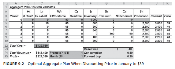
Compared with the base case, offering a discount in January results in lower seasonal inventory, a somewhat lower total cost, and a higher total profit.

IMPACT OF OFFERING A PROMOTION IN APRIL Now, management considers the impact of offering the discount in April. To simulate this option in the spreadsheet Chapter8,9-examples, enter 1 in cell E24 (this sets promotion to be on) and 4 in cell E25 (this sets the promotion in Period 4—i.e., April). If Green Thumb offers the discount in April, the demand forecast is as shown in cells J5:J10 of Figure 9-3. The optimal aggregate plan is obtained by running Solver and is shown in Figure 9-3. Compared with discounting in January (Figure 9-2), discounting in April requires more capacity (in terms of workforce) and leads to a greater buildup of seasonal inventory and larger stockouts because of the big jump in demand in April. With a discount in April, we have the following:

Total cost over planning horizon = $ 438,920

Revenue over planning horizon = $ 650,140

Profit over planning horizon = $ 211,220

Observe that a price promotion in January results in a higher supply chain profit, whereas a promotion in April results in a lower supply chain profit, compared with the base case of not running a promotion. As a result of the S&OP process, Red Tomato and Green Thumb decide to offer the discount in the off-peak month of January. Even though revenues are higher when the discount is offered in April, the increase in operating costs makes it a less profitable option. A promotion in January allows Red Tomato and Green Thumb to increase the profit they can share.

Note that this analysis is possible only because the retailer and manufacturer have an S&OP process that facilitates collaboration during the planning phase. This conclusion supports our earlier statement that it is not appropriate for a supply chain to leave pricing decisions solely in the domain of retailers and aggregate planning solely in the domain of manufacturers, with each having individual forecasts. It is crucial that forecasts, pricing, and aggregate planning be coordinated in a supply chain.

The importance of a collaborative S&OP process is further supported by the fact that the optimal action is different if most of the demand increase comes from market growth or stealing market share rather than from forward buying. We now illustrate the scenario in which a discount leads to a large increase in consumption.

3. When to Offer a Promotion If Discount Leads to a Large Increase in consumption

Reconsider the situation in which discounting a unit from $40 to $39 results in the period demand increasing by 100 percent (instead of the 10 percent considered in the previous analysis) because of increased consumption or substitution. Further, 20 percent of each of the two following months’ demand is moved forward. The supply chain team wants to determine whether it is pref­erable to offer the discount in January or April under these conditions. To simulate this scenario, change the entry in cell H24 (increase in consumption) of spreadsheet Chapter8,9-examples from 0.10 (10 percent) to 1.00 (100 percent). Set the entry in cell E24 to 1 to set the promotion to be on. The base case when no promotion is offered remains unchanged as shown in Figure 9-1. We now repeat the analysis for the cases in which the promotion is offered in January (off-peak) and April (peak).

IMPACT OF OFFERING A PROMOTION IN JANUARY For a January promotion, set the entry in cell E25 to 1 (Period 1, January). If the discount is offered in January, the January demand fore­cast is obtained as (1,600 X 2) + [0.2 X (3,000 + 3,200)] = 4,440. This is much higher than the same forecast in Figure 9-2 because we have assumed that consumption in the promotion month increases by 100 percent, rather than the 10 percent assumed earlier. The demand forecast for a January promotion with a large increase in consumption is shown in cells J5:J10 of Figure 9-4.

The optimal aggregate plan is obtained using Solver and is shown in Figure 9-4.

With a discount in January the team obtains the following:

Total cost over planning horizon = $ 456,880

Revenue over planning horizon = $ 699,560

Profit over planning horizon = $ 242,680

Observe that a January promotion when the consumption increase is large results in a higher profit than the base case (Figure 9-1).

IMPACT OF OFFERING A PROMOTION IN APRIL For an April promotion, set the entry in cell E25 to 4 (Period 4, April). If the discount is offered in April, the April demand forecast is obtained as (3,800 X 2) + [0.2 X (2,200 + 2,200)] = 8,480. With a promotion in April and a large increase in consumption, the April peak is much higher in Figure 9-5 compared with peak demand in Figure 9-4 (with a January promotion). For an April promotion with a large increase in consump­tion, the resulting demand forecast is as shown in cells J5:J10 of Figure 9-5. The optimal aggre­gate plan is obtained using Solver and is shown in Figure 9-5.

With a discount in April, the team obtains the following:

Total cost over planning horizon = $ 536,200

Revenue over planning horizon = $ 783,520

Profit over planning horizon = $ 247,320

When comparing Figures 9-5 and 9-4, observe that with an April promotion (Figure 9-5), there are no layoffs and the full workforce is maintained. The April promotion requires a much higher level of seasonal inventory and also uses stockouts and subcontracting to a greater extent than a January promotion. It is clear that costs will go up significantly with an April promotion. The interesting observation is that revenues go up even more (because of a larger consumption increase), making overall profits higher with an April promotion compared with a January pro­motion. As a result, when the increase in consumption from discounting is large and forward buying is a small part of the increase in demand from discounting, the supply chain is better off offering the discount in the peak-demand month of April, even though this action significantly increases supply chain costs.

Exactly as discussed earlier, the optimal aggregate plan and profitability can also be deter­mined for the case in which the unit price is $31 (enter 31 in cell H23) and the discounted price is $30. The results of the various instances are summarized in Table 9-3.

From the results in Table 9-3, we can draw the following conclusions regarding the impact of promotions:

1. As seen in Table 9-3, average inventory increases if a promotion is run during the peak period and decreases if the promotion is run during the off-peak period.
2. Promoting during a peak-demand month may decrease overall profitability if there is a small increase in consumption and a significant fraction of the demand increase results from a forward buy. In Table 9-3, observe that running a promotion in April decreases profitability when forward buying is 20 percent and the demand increase from increased consumption and substitu­tion is 10 percent.

3. As the consumption increase from discounting grows and forward buying becomes a smaller fraction of the demand increase from a promotion, it is more profitable to promote dur­ing the peak period. From Table 9-3, for a sale price of $40, it is optimal to promote in the off- peak month of January, when forward buying is 20 percent and increased consumption is 10 percent. When forward buying is 20 percent and increased consumption is 100 percent, however, it is optimal to promote in the peak month of April.
4. As the product margin declines, promoting during the peak-demand period becomes less profitable. In Table 9-3, observe that for a unit price of $40, it is optimal to promote in the peak month of April when forward buying is 20 percent and increased consumption is 100 per­cent. In contrast, if the unit price is $31, it is optimal to promote in the off-peak month of January for the same level of forward buying and increase in consumption.

A key point from the Red Tomato supply chain examples we have considered in this chap­ter is that when a firm is faced with seasonal demand, it should use a combination of pricing (to manage demand) and production and inventory (to manage supply) to improve profitability. The precise use of each lever varies with the situation. This makes it crucial that enterprises in a sup­ply chain coordinate both their forecasting and planning efforts through an S&OP process. Only then are profits maximized.

Source: Chopra Sunil, Meindl Peter (2014), Supply Chain Management: Strategy, Planning, and Operation, Pearson; 6th edition.