ARMAX Models by using Stata

Earlier in this chapter we saw that an OLS regression of ncdctemp on four lagged predictors gave a good fit to observed temperature values (Figure 12.2), as well as physically plausible parameter estimates. A Durbin-Watson test found significant autocorrelation among the residuals, however, which undermines the OLS t and F tests. ARMAX (autoregressive moving average with exogenous variables) modeling provides a better approach for this problem.

A similar ARMAX model with one-month lagged predictors and ARIMA(1,0,1) disturbances proves to fit well.

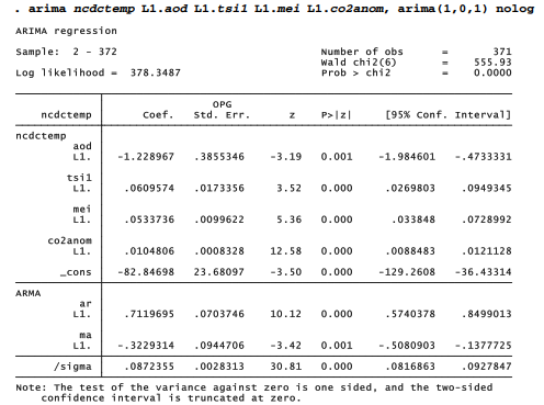
In this model y_t , or ncdctemp at time t, is a function of the lag-1 values of predictor variables x₁ through x₄ (aod through co2anom) and a disturbance (u_t):

The disturbance at time t (u_t) is related to the lag-1 disturbance (u_t-1) and to lag-1 and time t random errors (e_t-1 and e, ):

Coefficients on all four predictors, and on the AR and MA terms, are statistically significant at p < .01 or better. ncdctemp itself is not stationary, and does not need to be for this analysis. Indeed, its nonstationarity is the focus of research. Residuals from a successful model, however, should resemble white noise, a covariance stationary process. That is the case here: a portmanteau Q test gives p = .60 for residuals up to lag 25).

. predict ncdchat2

. label variable ncdchat2 “Predicted from volcanoes, solar, ENSO & CO2”

. predict ncdcres2, resid

. label variable ncdcres2 “NCDC residuals from ARMAX model”

. corrgram ncdcres2, lags(25)

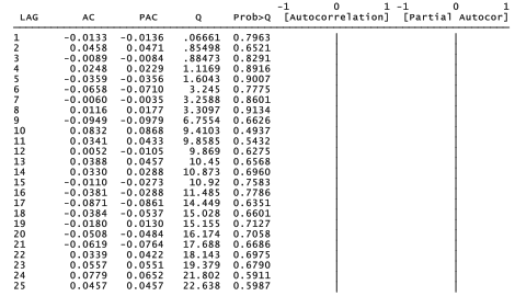
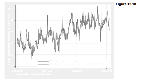
Figure 12.18 visualizes the close fit between data and the ARMAX model. The model explains about 77% of the variance in temperature anomalies. These ARMAX results support a general conclusion from our earlier OLS exploration: the multi-decade upward trend in temperatures cannot be explained without taking human drivers into account. The apparent slowdown in warming over the last decade, on the other hand, is better explained by natural drivers — La Niña and low solar irradiance.

Up to this point we have dealt only with one of the three temperature indexes in Climate.dta. This index is produced by the National Climate Data Center (NCDC) of the U.S. National Oceanic and Atmospheric Administration (NOAA). NCDC calculates its index based on surface temperature measurements taken at thousands of stations around the globe. NASA’s Goddard Institute for Space Studies produces its own temperature index (called GISTEMP), also based on surface station measurements but with better coverage of high-latitude regions.

The third temperature index in Climate.dta has a different basis. Researchers at the University of Alabama, Huntsville (UAH) calculate their global index from indirect satellite measurements of the upper troposphere, a region of Earth’s atmosphere up to about 4 km altitude. The satellite- based estimates show greater month-to-month variability, and are more sensitive to El Nino and La Nina events. They provide an alternative perspective on global temperature trends, consistent with the surface records but with some differences in details. How do these differences manifest when we model uahtemp with the same ARMAX approach used with ncdctemp?

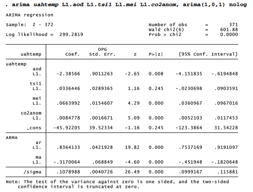
Coefficients in the NCDC and UAH models, as well as NASA (not shown), all have the same sign, consistent with physical understanding. In all three models, CO₂ anomaly proves the strongest predictor of temperature, and MEI second strongest. MEI exerts relatively more influence in the UAH model, as expected with satellite data. Volcanic aerosols also have stronger effects on the UAH index, while solar irradiance exhibits weaker effects. Reflecting the higher variability of satellite-based estimates, the model explains only 70% of the variance in uahtemp, compared with 77% for ncdctemp. However, the residuals pass tests for white noise (p = .65), and a plot of observed and predicted values shows a good visual fit (Figure 12.19).

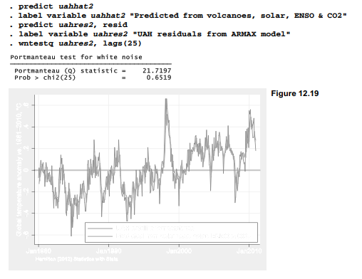
Satellite temperature records are a more recent development than weather-station records, so UAH temperature anomalies are calculated from a 1981-2010 baseline instead of 1901-2000 as done by NCDC. The recent baseline shifts the zero point for the UAH anomalies higher, as can be seen comparing Figure 12.19 with 12.18. Both series exhibit similar trends, however — about .16 °C/decade for NCDC (or NASA) over this period, or .15 °C/decade for UAH.

The conclusions from these simple ARMAX models generally agree with those from more sophisticated analyses by Foster and Rahmstorf (2011). Their approach involved searching for optimal lag specifications, in contrast to the arbitrary choice of 1-month lags for all predictors here. Foster and Rahmstorf also include trigonometric functions (a second-order Fourier series) to model residual annual cycles in the data. Time rather than CO₂ concentration was included among their predictors, to highlight temporal trends, but these trends are interpreted as human- caused. In principle those human causes could include other greenhouse gases besides CO₂, and other activities such as deforestation, land cover change or ozone depletion that are not captured by our co2anom variable, so a CO₂ causal interpretation may be overly simple. In practice, however, CO₂ has increased so directly with time (Figure 12.10) that using either time or CO₂ as a predictor will give similar results.

Source: Hamilton Lawrence C. (2012), Statistics with STATA: Version 12, Cengage Learning; 8th edition.