Artifact Corrections to Consider in Meta-Analysis

Hunter and Schmidt (2004; see also Schmidt, Le, & Oh, 2009) suggest several corrections to methodological artifacts of primary studies. These corrections involve unreliability of measures, poor validity of measured variables, arti­
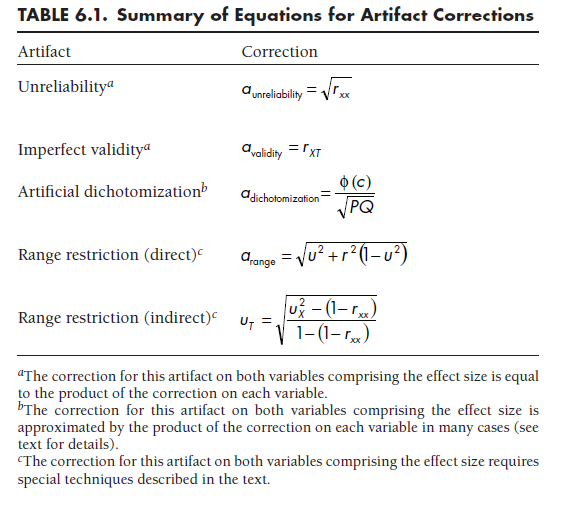
ficial dichotomization of continuous variables, and range restriction of vari­ables. Next I describe the conceptual justification and computational details of each of these corrections. The computations of these artifact corrections are summarized in Table 6.1.

Before turning to these corrections, however, let us consider the general formula for all artifact corrections. The corrected effect size (e.g., r, g, o), which is the estimated effect size if there were no study artifacts, is a function of the effect size observed in the study divided by the total artifact correc- tion¹:

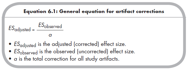
Here, a is the total correction for all study artifacts and is simply the product of the individual artifacts described next (i.e., a = a1 * a2 * . . . , for the first, second, etc., artifacts for which you wish to correct).² Each individual artifact (ai) and the total product of all artifacts (a) have values that are 1.0 (no artifact bias) or less (with the possible exception of the correction for range restriction, as described below). The values of these artifacts decrease (and adjustments therefore increase) as the methodological limitations of the studies increase (i.e., larger problems, such as very low reliability, result in smaller values of a and larger corrections).

Artifact adjustments to effect sizes also require adjustments to standard errors. Because standard errors represent the imprecision in estimates of effect sizes, it makes conceptual sense that these would increase if you must make an additional estimate in the form of how much to correct the effect size. Specifically, the standard errors of effect sizes (e.g., r, g, or o; see Chap­ter 5) are also adjusted for artifact correction using the following general formula:

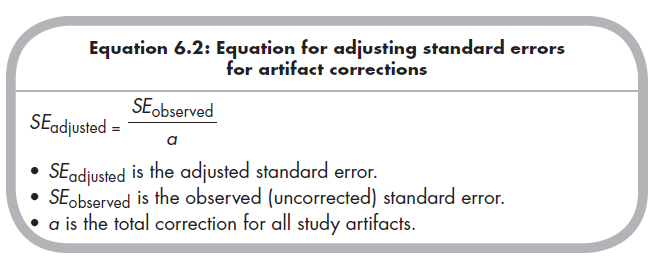
The one exception to this equation is when one is correcting for range restriction. This correction represents an exception to the general rule of Equation 6.2 because the effect size is used in the computation of a, the arti­fact correction (see Equations 6.7 and 6.8). In this case of correcting for range restriction, you multiply a_rang_e by ES_adj_usted/ES_ob_served prior to correcting the standard error.

1. Corrections for Unreliability

This correction is for unreliability of measurement of the variables comprising the effect sizes (e.g., variables X and Y that comprise a correlation). Unreliabil­ity refers to nonsystematic error in the measurement process (contrast with systematic error in measurement, or poor validity, described in Section 6.2.4).

Reliability, or the repeatability of a measure (or the part that is not unreliable), can be indexed in at least three ways. Most commonly, reliability is considered in terms of internal consistency, representing the repeatability of measurement across different items of a scale. This type of reliability is indexed as a func­tion of the associations among items of a scale, most commonly through an index called Cronbach’s coefficient alpha, a (Cronbach, 1951; see, e.g., DeVel- lis, 2003). Second, reliability can be evaluated in terms of agreement between multiple raters or reporters. This interrater reliability can be evaluated with the correlation between sets of continuous scores produced by two raters (or average correlations among more than two raters) or with Cohen’s kappa (k) representing agreement between categorical assignment between raters (for a full description of methods of assessing interrater reliability, see von Eye & Mun, 2005). A third index of reliability is the test—retest reliability. This test- retest reliability is simply the correlation (r) between repeated measurements, with the time span between measurements being short enough that the con­struct is not expected to change during this time. Because all three types of reliability have a maximum of 1 and a minimum of 0, the relation between reliability and unreliability can be expressed as reliability = 1 – unreliability.

Regardless of whether reliability is indexed as internal consistency (e.g., Cronbach’s a), interrater agreement (r or k), or test-retest reliability (r), this reliability impacts the magnitude of effect sizes that a study can find. If reliability is high (e.g., near perfect, or close to 1) for the measurement of two variables, then you expect that the association (e.g., correlation, r) the researcher finds between these variables will be an unbiased estimate of the actual (latent) population effect size (assuming the study does not contain other artifacts described below). However, if the measurement of one or both variables comprising the association of interest is low (reliability far below 1, maybe even approaching 0), then the maximum (in terms of absolute value of positive or negative associations) effect size the researcher might detect is substantially lower than the true population effect size. This is because the correlation (or any other effect size) between the two variables of inter­est is being computed not only from the true association between the two constructs, but also between the unreliable aspects of each measure (i.e., the noise, which typically is not correlated across the variables).

If you know (or at least have a good estimate of) the amount of unre­liability in a measure, you can estimate the magnitude of this effect size attenuation. This ability is also important for your meta-analysis because you might wish to estimate the true (disattenuated) effect size from a primary study reporting an observed effect size and the reliability of measures. Given the reliability for variables X and Y, with these general reliabilities denoted as
r_xx and ryy, you can estimate the corrected correlation (i.e., true correlation between constructs X and Y) using the following artifact adjustment (Baugh, 2002; Hunter & Schmidt, 2004, pp. 34-36):

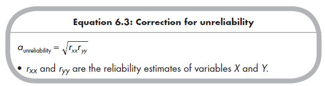
As described earlier (see Equation 6.1), you estimate the true effect size by dividing the observed effect size by this (and any other) artifact adjust­ment. Similarly, you increase the standard error (SE) of this true effect size estimate to account for the additional uncertainty of this artifact correction by dividing the standard error of the observed effect size (formulas provided in Chapter 5) by this (and any other) artifact adjustment (see Equation 6.2).

An illustration using a study from the ongoing example meta-analysis (Card et al., 2008) helps clarify this point. This study (Hawley, Little, & Card, 2007) reported a bivariate correlation between relational aggression and rejection of r = .19 among boys (results for boys and girls were each cor­rected and later combined). However, the measures of both relational aggres­sion and rejection exhibited marginal internal consistencies (a_s = .82 and .81, respectively), which might have contributed to an attenuated effect size of this correlation. To estimate the adjusted (corrected) correlation, I compute first and

The standard error of Fisher’s transformation of this uncorrected correlation is .0498 (based on N = 407 boys in this study); I also adjust this standard error to se _adjusted = .0498 _ _₀₆₁₀. This larger standard error represents the greater imprecision in the adjusted effect size estimated using this correction for unreliability.

This artifact adjustment (Equation 6.3) can also be used if you wish to correct for only one of the variables being correlated (e.g., correction for X but not Y). This may be the preference because the meta-analyst assumes that one of the variables is measured without error, because the primary studies fre­quently do not report reliability estimates of one of the variables, or because the meta-analyst is simply not interested in one of the variables.³ If you are interested in correcting for unreliability in one variable, then you implicitly assume that the reliability of the other variable is perfect. In other words, correction for unreliability in only one variable is equivalent to substituting 1.0 for the reliability of the other variable in Equation 6.3, so this equation simplifies to the artifact correction being the square root of the reliability of the single variable.

Before ending discussion of correction for unreliability, I want to men­tion the special case of latent variable associations. These latent variable asso­ciations include (1) correlations between factors from an exploratory factor analysis with oblique factor rotation (e.g., direct oblimin, promax), and (2) correlations between constructs in confirmatory factor analysis models.⁴ You should remember that these latent correlations are corrected for measure­ment error; in other words, the reliabilities of the latent variable are perfect (i.e., 1.0). Therefore, these latent correlations are treated as effect sizes already corrected for unreliability, and you should not further correct these effect sizes using Equation 6.3. This point can be confusing because many primary studies will report internal consistencies for these scales; but these internal consistencies are relevant only if the study authors had conducted manifest variable analyses (e.g., using summed scale scores) with these measures.

2. Corrections for Imperfect Validity

The validity of a measure refers to the systematic overlap between the mea­sure and the intended construct (i.e., the thing the measure is meant to mea­sure). It is important to distinguish between validity and reliability. Reli­ability, described earlier, refers to the repeatability of a measure across items, raters, or occasions; high reliability is indicated by different items, raters, or occasions of measurement having high correspondence (i.e., being highly correlated). However, reliability does not tell us whether we are measuring what we intend to measure, but only that we are measuring the same thing (whatever it may be) consistently. In contrast, validity refers to the consis­tency between the measure and the construct. For instance, “Does a par­ticular peer nomination instrument truly measure victimization?”, “Does a parent-report scale really measure depression?”, and “Does a particular IQ test measure intelligence?” are all questions involving validity. Low valid­ity means that the measure is reliably measuring something other than the intended construct. Reliability and validity are entirely independent phe­nomena: A scale can have high reliability and low validity, and another scale can have low reliability and high validity (if one assesses validity by correct­ing for attenuation due to unreliability, as in latent variable modeling; Little, Lindenberger, & Nesselroade, 1999).

You can conceptualize a measure’s degree of validity as the disattenu- ated correlation between the measure and the construct. In other words, the validity of a measure (X) in assessing a construct (T) is txt when the mea­sure is perfectly reliable. If the effect size of interest in your meta-analysis is the association between the true construct (T) and some other variable (Y; assuming for the moment that this variable is measured with perfect valid­ity), then the association you are interested in might be represented as tty (you could also apply this correction to other effect sizes, but the use of cor­relations here facilitates understanding). Therefore, the observed association between the measure (X) and the other variable (Y) is equal to the product of the validity of the measure and the association of the construct with the other variable, txy = txt * tty. To identify the association between the con­struct (T) and the other variable (Y), which is what you are interested in, you can rearrange this expression to tty = txy/txt In other words, the adjustment for imperfect validity in a study is:

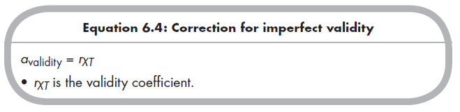
Here, txt represents the validity coefficient or disattenuated (for mea­surement unreliability) correlation between the measure (X) and intended construct (T).

This adjustment is mathematically simple, yet its use contains two chal­lenges. The first challenge is that this adjustment assumes that whatever is specific to the measure (X) that is not part of the construct (T) is uncorrelated with the other variable (Y). In other words, the reliable but invalid portion of the measure (e.g., method variance) is assumed to not be related to the other variable of interest (either the construct Ty or its measure, Xy). The second challenge in applying this adjustment is simply in obtaining an estimate of the validity coefficient (xt). This validity will almost never be reported in the primary studies of the meta-analysis (if a study contained this more valid variable, then you would simply use effect sizes from this variable rather than the invalid proxy). Most commonly, you need to obtain the validity coefficient from another source, such as from validity studies of the measure (X). When using the validity coefficient from other studies, however, you must be aware of both (unreliable) sampling error in the magnitude of this correlation and (reliable but unknown) differences in this correlation between the validity population and that of the particular primary study you are coding. For these reasons, I suspect that many fields will not contain adequate information to obtain a good estimate of the validity coefficient, and therefore this artifact adjustment may be difficult to use.

3. Corrections for Artificial Dichotomization

It is well known that artificial dichotomization of a variable that is naturally continuous attenuates associations that this variable has with others, yet this practice is all too common in primary research (see MacCallum et al., 2002). An important distinction is whether a variable is artificially dichotomized or truly dichotomous. When analyzing associations between two continu­ous variables (typically using r as an index of effect size; see Chapter 5), you might find that a primary study artificially dichotomized one of the vari­ables in one of many possible ways, including median splits, splits at some arbitrary level (e.g., one standard deviation above the mean), or at some rec­ommended cutoff level (e.g., at a level where a variable of maladjustment is considered “clinically significant”). Or you might find that the primary study dichotomized both variables of interest (again, through median splits, etc.). Finally, you might be interested in the extent to which two groups (a natu­rally dichotomous variable) differ on a continuous variable, which is dichoto­mized in some studies (e.g., the studies report the percentages of each group that have “clinically significant” levels of a maladjustment variable). In each of these cases, you need to recognize that the dichotomization of variables in the primary studies is artificial; that it does not represent the true continuous nature of the variable.

Corrections for one variable that is artificially dichotomized are straight­forward. You need only to know the numbers, proportion, or percentages of individuals in the two artificial groups. Based on this information, the arti­fact adjustment for dichotomization of one variable is (Hunter & Schmidt, 1990; Hunter & Schmidt, 2004, p. 36; MacCallum et al., 2002):

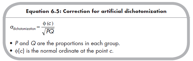
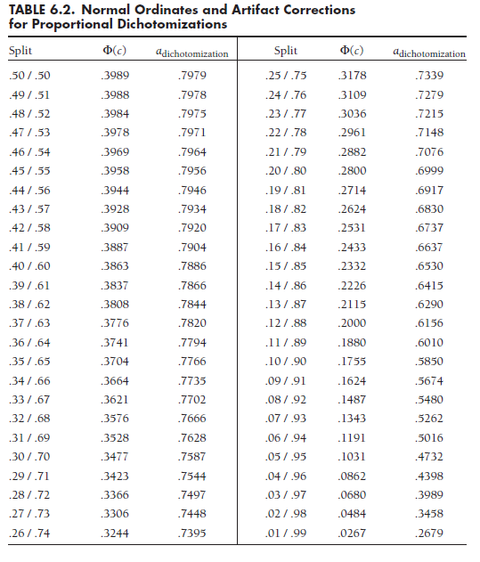
The numerator, Φ(c), is the normal ordinate at the point c that divides the standard normal distribution into proportions P and Q. Because this value is unfamiliar to many, I have listed values of Φ(c), as well as the artifact adjustment for dichotomization of one variable (fldichotomizaticm), for various proportional splits in Table 6.2.

To illustrate this correction using the ongoing example (Card et al., 2008), I consider a study by Crick and Grotpeter (1995). Here, the authors artificially dichotomized the relational aggression variable by classifying children with scores one deviation above the mean as relationally aggressive and the rest as not relationally aggressive. Of the 491 children in the study, 412 (83.9%) were thus classified as not aggressive and 79 (16.1%) as relationally aggressive. The numerator of Equation 6.5 for this example is found in Table 6.2 to be .243. The denominator for this example is .368. Therefore, adichotomization = .243/.368 = .664 (accepting some rounding error), as shown in Table 6.2. For this example, the uncorrected correlation between relational aggression and rejection was .16 (computed from F(1,486) = 12.3) and the standard error of Zr was .0453 (from N = 491). The adjustment for artificial dichotomization yields radjusted = .16/.664 = .24 and SEadjusted = .0453/.664 = .0682. (Note that this adjustment is only for artificial dichotomization; we ultimately corrected for unreliability as well, which is why this effect size differs from that used in our analyses and used later.)

If both of two continuous variables are dichotomized, the correction becomes complex (specifically, you must compute a tetrachoric correlation; see Hunter & Schmidt, 1990). Fortunately, a simple approximation holds in most cases you are likely to encounter. Specifically, the artifact adjustment for two artificially dichotomized variables can be approximated by:

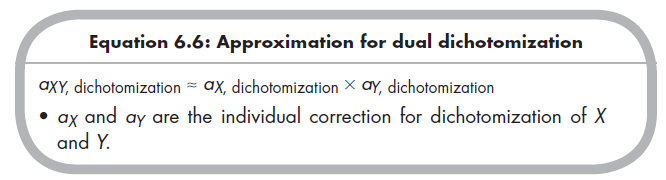
In other words, the artifact adjustment for two variables is approximated by the product of each adjustment for the dichotomization of each variable. The feasibility of this approximation depends on the extremity of the dichot- omization split and the corrected correlation (r_adjusted). Hunter and Schmidt (1990) showed that this approximation is reasonable when (1) one of the vari-ables has a median (P = .50) split and the corrected correlation is less than .70; (2) one of the variables has an approximately even split (.40 < P < .60) and the corrected correlation is less than .50; or (3) neither of the variables has extreme splits (.20 < P < .80) and the corrected correlation is less than .40. If any of these conditions apply, then this approximation is reasonably accurate (less than 10% bias). If the dichotomizations are more extreme or the corrected correlations are very large, then you should use the tetrachoric correlation described by Hunter and Schmidt (1990).

4. Corrections for Range Restriction

Estimates of associations between continuous variables are attenuated in studies that fail to sample the entire range of population variability on these variables. As an example (similar to that described by Hunter, Schmidt, & Le, 2006), it might be the case that GRE scores are strongly related to success in graduate school, but because only applicants with high GRE scores are admitted to graduate school, a sample of graduate students might reveal only small correlations between GRE scores obtained and some index of success (i.e., this association is attenuated due to restriction in range). This does not necessarily mean that there is only a small association between GRE scores and graduate school success, at least if we define our population as all poten­tial graduate students rather than just those admitted. Instead, the estimated correlation between GRE scores and graduate school success is attenuated (reduced) due to the restricted range of GRE scores for those students about whom we can measure success. Aside from GRE scores and graduate school success, it is easy to think of numerous other research foci for which restric­tion of range may occur: Studies of correlates of job performance are limited to those individuals hired, educational research too often includes only chil­dren in mainstream classrooms, and psychopathology research might only sample individuals who seek psychological services. Combination and com­parison of studies using samples of differing ranges might prove difficult if you do not correct for restrictions in range of one or both variables under consideration.

The first step in adjusting effect sizes for range restriction in one vari­able is to define some amount of typical (standard) deviation of that vari­able in the population and then determine the amount of deviation within the primary study sample relative to this reference population. This ratio of study (restricted) deviation to reference (unrestricted) standard deviation is denoted as u = 5D_study/SD_ref_erence (Hunter & Schmidt, 2004, p. 37). With some studies, determining this u may be straightforward. For example, if a study reports the standard deviation of the sample on an IQ test (e.g., 10) with a known population standard deviation (e.g., 15), then we could compare the sample range on IQ relative to the population range (e.g., u = 10/15 = 0.67).

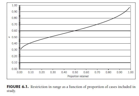
In other situations, the authors of primary studies select individuals scor­ing in the top or bottom of a certain percentile range (e.g., selection of those above the median of a variable for inclusion is equivalent to selecting the top 50th percentile). In these situations, it is possible to compute the amount that the range is restricted. Although such calculations are complicated (see Barr & Sherrill, 1999), Figure 6.1 shows the values of u given the proportion of individuals selected for the study. The x-axis of this figure represents the proportion of individuals included in the study (e.g., selection of all individu­als above the 10th percentile means retention of 0.90 of participants). It can be seen that the less selective a study is (i.e., a higher proportion is retained, shown on the right side of the figure), the less restricted the range (i.e., u approaches 1), whereas the more selective a study is (i.e., a lower proportion is retained, shown on the left side of the figure), the more restricted the range (i.e., u becomes smaller). Note that the computations on which Figure 6.1 is based assume a normal distribution of the variable within the reference population and are only applicable with one-sided truncated data (i.e., the research selected individuals based on their falling above or below a single score or percentile cutoff).

In other situations, however, it may be difficult to determine a good esti­mate of the sample variability relative to that of the population. Although a perfect solution likely does not exist, I suggest the following: Select primary studies from all included studies that you believe do not suffer restriction of range (i.e., those that were fully sampled from the population to which you wish to generalize). From these studies, estimate the population (i.e., unrestricted) standard deviation by meta-analytically combining standard deviations (see Chapter 7). Then use this estimate to compute the degree of range restriction (u) among studies in which participants were sampled in a restrictive way.

The artifact adjustment for range restriction is based on this ratio of the sample standard deviation relative to the reference population standard devi­ation (as noted: u = 5D_study/SD_reference) as well as the correlation reported in the study.⁵ Specifically, this adjustment is (Hunter & Schmidt, 2004, p. 37):

 

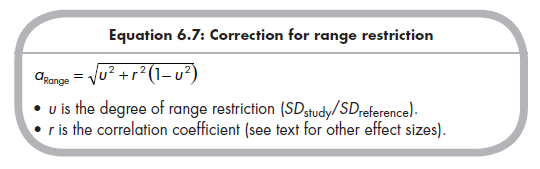
A unique aspect of this artifact adjustment for range restriction is that it can yield a values greater than 1.0 (in contrast to my earlier statement that these adjustments are always less than 1.0). The situation in which this can occur is when the sample range is greater than the reference population range (i.e., range enhancement). Although range enhancement is probably far less common than range restriction, this situation is possible in studies where individuals with extreme scores were intentionally oversampled.

A more complex situation is that of indirect range restriction (in contrast to the direct range restriction I have described so far). Here, the variables comprising the effect size (e.g., X and Y) were not used in selecting partici­pants, but rather a third variable (e.g., Z) that is related to one of the variables of interest was used for selection. If (1) the range of Z in the sample is smaller than that in the population, and (2) Z is associated with X or Y, then the effective impact of this selection is that the range of X or Y in the sample is indirectly restricted. Continuing the example I used earlier, imagine that we are interested in the association between IQ (X) and graduate school success (Y). Although students might not be directly selected based on IQ, the third variable GRE (Z) is correlated with IQ, and we therefore have indirect restric­tion in the range of IQ represented in the sample.

This situation of indirect range restriction may be more common than that of direct range restriction that I have previously described (Hunter et al., 2006). It is also more complex to correct. Although I direct readers inter­ested in a full explanation to other sources (Hunter & Schmidt, 2004, Ch. 3; Hunter et al., 2006; Le & Schmidt, 2006), I briefly describe this procedure. First, you need to consider both the sample standard deviation of the indi­rectly restricted variable (e.g., IQ, if GRE scores are used for selection and are associated with IQ) as well as the reliability of this restricted variable. You then compute an alternative value of u for use in Equation 6.7. Specifically, you compute this alternative ratio, denoted as uj by Hunter and Schmidt (2004; Hunter et al., 2006, p. 106) using the following formula:

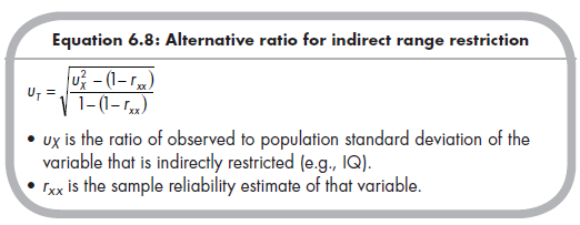
As mentioned, this alternative ratio uj is then applied as u in Equation 6.7.

Another situation of range restriction is that of restriction on both vari­ables comprising the effect size. In the example involving GRE scores and graduate school success, the sample may be restricted in terms of both selec­tion on GRE scores (i.e., only individuals with high scores are accepted into graduate schools) and graduate school success (e.g., those who are unsuccess­ful drop out of graduate programs). This is an example of range restriction on both variables of the effect size, or double-range restriction (also called “dou­bly truncated” by Alexander, Carson, Alliger, & Carr, 1987). Although no exact methods exist for simultaneously correcting range restriction on both variables (Hunter & Schmidt, 2004, p. 40), Alexander et al. (1987) proposed an approximation in which one corrects first for restriction in range of one variable and then for restriction of range on the second variable (using the r corrected for range restriction on the first variable in Equation 6.7). Alexan­der et al. (1987) show that this approximation is generally accurate for most situations meta-analysts are likely to encounter, and Hunter and Schmidt (2004) report that this approximation can be used to correct for either direct or indirect range restriction.

Source: Card Noel A. (2015), Applied Meta-Analysis for Social Science Research, The Guilford Press; Annotated edition.