Miscellaneous Effect Sizes in Meta-Analysis

As I hope is becoming increasingly clear, you can include a wide range of options for effect sizes in your meta-analyses. Although this section on miscellaneous effect sizes could include dozens of possibilities, I limit my description to two that seem especially useful: scale internal consistency and longitudinal change scores.

1. Scale Internal Reliability

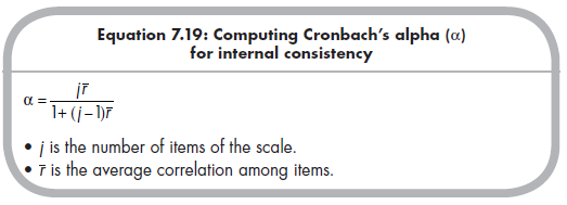
Internal consistency, or the internal reliability of a scale, indexes the magni­tude to which items of a scale are homogeneous. The most widely used index of this internal consistency is Cronbach’s alpha, a (Cronbach, 1951), which can be computed based on the number of items in a scale (j) and the average correlation among these items (r):

There are two situations in which you might be interested in meta­analyzing internal consistency. One situation was raised in Chapter 6—when I described the situation in which you wish to correct for unreliability but this estimate is not provided in some studies. In this situation, a meta-analytically derived mean or predicted variable (i.e., predicted by characteristics of the study) provides a reasonable estimate of internal consistency to use when correcting for the artifact of unreliability. A second situation is when the internal consistency is itself of interest. For instance, you might be interested in knowing the average internal consistency of a scale across multiple studies (i.e., the mean internal consistency), or you might be interested in the con­ditions under which internal consistency is higher or lower (i.e., moderator analyses across study characteristics). In both situations, meta-analysis of internal consistency estimates is valuable.

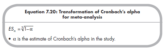
Although various methods of meta-analyzing reliability results have been proposed, I rely on the method described by Rodriguez and Maeda (2006) for Cronbach’s alpha. This approach is relatively simple, and Cronbach’s alpha is reported in most studies.⁸ This method relies on a transformation of Cron­bach’s alpha as the effect size (Rodriguez & Maeda, 2006):

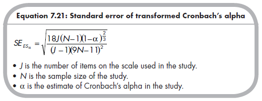
The standard error of this transformed internal consistency is a function of the number of items on the scale used in the study, the sample size, and the estimate of internal consistency itself (Rodriguez & Maeda, 2006):

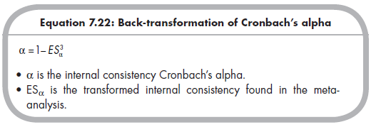
After computing the mean transformed internal consistency (as well as confidence interval limits or predicted values at different levels of modera­tors), you should back-transform results into the more interpretable Cron- bach’s alpha:

2. Longitudinal change Scores

Longitudinal change is of central interest in many areas. In developmental science, much attention is given to change across age, which is often studied using naturalistic longitudinal designs (see Little et al., 2009). Longitudinal change is also relevant to experimental and quasi-experimental research; for instance, you might be interested in changes in some index of functioning from before to after an intervention. Given this empirical interest in longi­tudinal change, it follows that you may be interested in meta-analytically combining and comparing this change across studies.

We can consider longitudinal change scores as indexing a two-variable association between time (X) and the variable that is potentially increas­ing or decreasing (Y). Because most studies that you might potentially meta- analyze treat time as a categorical variable (e.g., Waves 1 and 2 of a survey, pre- and postintervention scores),⁹ you can represent these change scores as
either standardized mean change (e.g., g) or unstandardized mean change (if all studies use the same scale for the Y variable). Because it is more likely that you will want to meta-analyze studies using different measures of Y, I focus only on the standardized mean change here (for a description of unstandard­ized mean change, see Lipsey & Wilson, 2001, pp. 42-44).

The standardized mean change effect size is defined by the following formula (Lipsey & Wilson, 2001, p. 44):

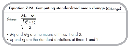
This equation is identical to that for the standardized mean difference (g) between independent groups shown in Chapter 5, if you recognize that the denominator is simply the pooled standard deviation across time. From this equation, you see that computing g_change from reported descriptive data is straightforward. One caveat is that you should be careful that the reported means and standard deviations at each time come from only the individuals who participated in both times. In other words, you need descriptive data from the nonattriting sample.¹⁰

Although most research reports will provide these descriptive data, you may find instances where they do not. If the primary study reports only a repeated-measures £-test or ANOVA (F-ratio), along with the correlation between Waves 1 and 2 (i.e., interindividual stability), you can use this infor­mation to compute g_change using the following equation (which was also pro­vided in Chapter 5):

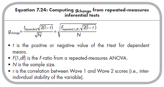
When using these equations, you should be sure that you are assigning the correct sign to the effect size. I strongly recommend always using positive scores to represent increases in the variable over time and negative scores to represent decreases. These equations also allow us to compute g_ch_ang_e from probability levels—be they exact (e.g., p = .034) or minimum effect sizes from a range (e.g., p < .05). Here, you simply look up the associated t or F value given the reported level of significance and degrees of freedom.

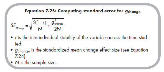
In addition to the effect size g_ch_ang_e, we also need to compute the stan­dard error of this estimate for weighting in our meta-analysis. As you would expect, the standard error is dependent on the sample size; but it is also dependent on the interindividual stability (r) of the variable across time. It is critical to find this information in the research report for accurately comput­ing this standard error; if it is not provided, you should seek to obtain this information from the study authors. The equation for the standard error for &h_ang_e is (Lipsey & Wilson, 2001, p. 44):

Before concluding this section on longitudinal change scores, I want to note that this approach is not limited only to longitudinal designs, even though that is where we are most likely to apply them. Instead, this approach can be used with any data that would typically be analyzed (in primary research) using paired-sample £-tests or two-group repeated-measures ANO- VAs. For example, this effect size would be appropriate in treatment stud­ies where individuals are matched into pairs, and then randomly assigned to treatment versus control groups (see e.g., Shadish et al., 2002, p. 118). Similarly, this effect size would be useful when meta-analyzing dyadic data in which individuals are interdependently linked, such as studies consider­ing differences between husbands and wives or between older and younger siblings (see Kenny, Kashy, & Cook, 2006). Although these types of studies are likely less common in most fields, you can keep these possibilities in mind.

Source: Card Noel A. (2015), Applied Meta-Analysis for Social Science Research, The Guilford Press; Annotated edition.