Choosing Firm’s Output in the Long Run

In the short run, one or more of the firm’s inputs are fixed. Depending on the time available, this may limit the flexibility of the firm to adapt its production process to new technological developments, or to increase or decrease its scale of operation as economic conditions change. In contrast, in the long run, a firm can alter all its inputs, including plant size. It can decide to shut down (i.e., to exit the industry) or to begin producing a product for the first time (i.e., to enter an industry). Because we are concerned here with competitive markets, we allow for free entry and free exit. In other words, we are assuming that firms may enter or exit without legal restriction or any special costs associated with entry. (Recall from Section 8.1 that this is one of the key assumptions underlying perfect competition.) After analyzing the long-run output decision of a profit-maximizing firm in a competitive market, we discuss the nature of competitive equilibrium in the long run. We also discuss the relationship between entry and exit, and economic and accounting profits.

1. Long–Run Profit Maximization

Figure 8.13 shows how a competitive firm makes its long-run, profit-maximizing output decision. As in the short run, the firm faces a horizontal demand curve. (In Figure 8.13 the firm takes the market price of $40 as given.) Its short-run average (total) cost curve SAC and short-run marginal cost curve SMC are low enough for the firm to make a positive profit, given by rectangle ABCD, by producing an output of q1, where SMC = P = MR. The long-run average cost curve LAC reflects the presence of economies of scale up to output level q2 and diseconomies of scale at higher output levels. The long-run marginal cost curve LMC cuts the long-run average cost from below at q2, the point of minimum long-run average cost.

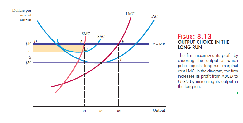
If the firm believes that the market price will remain at $40, it will want to increase the size of its plant to produce at output q3, at which its long-run marginal cost equals the $40 price. When this expansion is complete, the profit margin will increase from AB to EF, and total profit will increase from ABCD to EFGD. Output q3  is profit-maximizing because at any lower output (say, q2), the marginal revenue from additional production is greater than the marginal cost. Expansion is, therefore, desirable. But at any output greater than q3, marginal cost is greater than marginal revenue. Additional production would therefore reduce profit. In summary, the long-run output of a profit-maximizing competitive firm is the point at which long-run marginal cost equals the price.

Note that the higher the market price, the higher the profit that the firm can earn. Correspondingly, as the price of the product falls from $40 to $30, the profit also falls. At a price of $30, the firm’s profit-maximizing output is q2, the point of long-run minimum average cost. In this case, because P = ATC, the firm earns zero economic profit.

2. Long–Run Competitive Equilibrium

For an equilibrium to arise in the long run, certain economic conditions must prevail. Firms in the market must have no desire to withdraw at the same time that no firms outside the market wish to enter. But what is the exact relationship between profitability, entry, and long-run competitive equilibrium? We can see the answer by relating economic profit to the incentive to enter and exit a market.

ACCOUNTING PROFIT AND ECONOMIC PROFIT As we saw in Chapter 7, it is important to distinguish between accounting profit and economic profit. Accounting profit is measured by the difference between the firm’s revenues and its cash flows for labor, raw materials, and interest plus depreciation expenses. Economic profit takes into account opportunity costs. One such opportunity cost is the return to the firm’s owners if their capital were used elsewhere. Suppose, for example, that the firm uses labor and capital inputs; its capital equipment has been purchased. Accounting profit will equal revenues R minus labor cost wL, which is positive. Economic profit p, however, equals revenues R minus labor cost wL minus the capital cost, rK:

As we explained in Chapter 7, the correct measure of capital cost is the user cost of capital, which is the annual return that the firm could earn by investing its money elsewhere instead of purchasing capital, plus the annual depreciation on the capital.

ZERO ECONOMIC PROFIT When a firm goes into a business, it does so in the expectation that it will earn a return on its investment. A zero economic profit means that the firm is earning a normal—i.e., competitive—return on that investment. This normal return, which is part of the user cost of capital, is the firm’s opportunity cost of using its money to buy capital rather than investing it elsewhere. Thus, a firm earning zero economic profit is doing as well by investing its money in capital as it could by investing elsewhere—it is earning a competitive return on its money. Such a firm, therefore, is performing adequately and should stay in business. (A firm earning a negative economic profit, however, should consider going out of business if it does not expect to improve its financial picture.)

As we will see, in competitive markets economic profit becomes zero in the long run. Zero economic profit signifies not that firms are performing poorly, but rather that the industry is competitive.

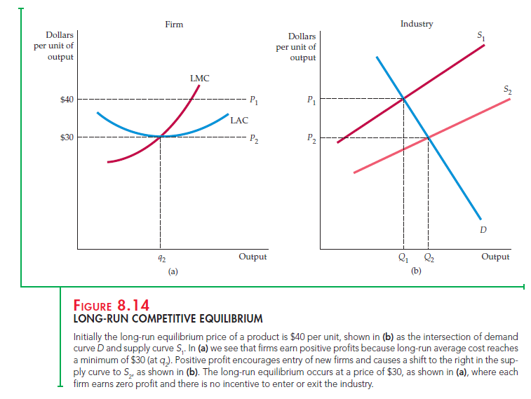
ENTRY AND EXIT Figure 8.13 shows how a $40 price induces a firm to increase output and realize a positive profit. Because profit is calculated after subtracting the opportunity cost of capital, a positive profit means an unusually high return on a financial investment, which can be earned by entering a profitable industry. This high return causes investors to direct resources away from other industries and into this one—there will be entry into the market. Eventually the increased production associated with new entry causes the market supply curve to shift to the right. As a result, market output increases and the market price of the prod- uct falls.7  Figure 8.14 illustrates this. In part (b) of the figure, the supply curve has shifted from S1 to S2, causing the price to fall from P1 ($40) to P2 ($30). In part (a), which applies to a single firm, the long-run average cost curve is tangent to the horizontal price line at output q2.

A similar story would apply to exit. Suppose that each firm’s minimum long-run average cost remains $30 but the market price falls to $20. Recall our discus-sion earlier in the chapter; absent expectations of a price change, the firm will leave the industry when it cannot cover all of its costs, i.e., when price is less than average variable cost. But the story does not end here. The exit of some firms from the market will decrease production, which will cause the market supply curve to shift to the left. Market output will decrease and the price of the product will rise until an equilibrium is reached at a break-even price of $30. To summarize:

In a market with entry and exit, a firm enters when it can earn a positive long- run profit and exits when it faces the prospect of a long-run loss.

When a firm earns zero economic profit, it has no incentive to exit the indus- try. Likewise, other firms have no special incentive to enter. A long-run com- petitive equilibrium occurs when three conditions hold:

1. All firms in the industry are maximizing profit.
2. No firm has an incentive either to enter or exit the industry because all firms are earning zero economic profit.
3. The price of the product is such that the quantity supplied by the industry is equal to the quantity demanded by consumers.

The dynamic process that leads to long-run equilibrium may seem puzzling. Firms enter the market because they hope to earn a profit, and likewise they exit because of economic losses. In long-run equilibrium, however, firms earn zero economic profit. Why does a firm enter a market knowing that it will eventually earn zero profit? The answer is that zero economic profit represents a competitive return for the firm’s investment of financial capital. With zero economic profit, the firm has no incentive to go elsewhere because it cannot do better financially by doing so. If the firm happens to enter a market sufficiently early to enjoy an economic profit in the short run, so much the better. Similarly, if a firm exits an unprofitable market quickly, it can save its investors money. Thus the concept of long-run equilibrium tells us the direction that a firm’s behavior is likely to take.

FIRMS HAVING IDENTICAL COSTS To see why all the conditions for long-run equilibrium must hold, assume that all firms have identical costs. Now consider what happens if too many firms enter the industry in response to an opportu- nity for profit. The industry supply curve in Figure 8.14(b) will shift further to the right, and price will fall below $30—say, to $25. At that price, however, firms will lose money. As a result, some firms will exit the industry. Firms will con- tinue to exit until the market supply curve shifts back to S2. Only when there is no incentive to exit or enter can a market be in long-run equilibrium.

FIRMS HAVING DIFFERENT COSTS Now suppose that all firms in the indus- try do not have identical cost curves. Perhaps one firm has a patent that lets it produce at a lower average cost than all the others. In that case, it is consistent with long-run equilibrium for that firm to earn a greater accounting profit and to enjoy a higher producer surplus than other firms. As long as other investors and firms cannot acquire the patent that lowers costs, they have no incentive to enter the industry. Conversely, as long as the process is particular to this product and this industry, the fortunate firm has no incentive to exit the industry.

The distinction between accounting profit and economic profit is important here. If the patent is profitable, other firms in the industry will pay to use it (or attempt to buy the entire firm to acquire it). The increased value of the patent thus represents an opportunity cost to the firm that holds it. It could sell the rights to the patent rather than use it. If all firms are equally efficient otherwise, the eco- nomic profit of the firm falls to zero. However, if the firm with the patent is more efficient than other firms, then it will be earning a positive profit. But if the patent holder is otherwise less efficient, it should sell off the patent and exit the industry.

THE OPPORTUNITY COST OF LAND  There are other instances in which firms earning positive accounting profit may be earning zero economic profit. Suppose, for example, that a clothing store happens to be located near a large shopping center. The additional flow of customers can substantially increase the store’s accounting profit because the cost of the land is based on its historical cost. However, as far as economic profit is concerned, the cost of the land should reflect its opportunity cost, which in this case is the current market value of the land. When the opportunity cost of land is included, the profitability of the clothing store is no higher than that of its competitors.

Thus the condition that economic profit be zero is essential for the market to be in long-run equilibrium. By definition, positive economic profit represents an opportunity for investors and an incentive to enter an industry. Positive accounting profit, however, may signal that firms already in the industry pos- sess valuable assets, skills, or ideas, which will not necessarily encourage entry.

3. Economic Rent

We have seen that some firms earn higher accounting profit than others because they have access to factors of production that are in limited supply; these might include land and natural resources, entrepreneurial skill, or other creative tal- ent. In these situations, what makes economic profit zero in the long run is the willingness of other firms to use the factors of production that are in limited supply. The positive accounting profits are therefore translated into economic rent that is earned by the scarce factors. Economic rent is what firms are willing to pay for an input less the minimum amount necessary to buy it. In competitive markets, in both the short and the long run, economic rent is often positive even though profit is zero.

For example, suppose that two firms in an industry own their land outright; thus the minimum cost of obtaining the land is zero. One firm, however, is located on a river and can ship its products for $10,000 a year less than the other firm, which is inland. In this case, the $10,000 higher profit of the first firm is due to the $10,000 per year economic rent associated with its river location. The rent is created because the land along the river is valuable and other firms would be willing to pay for it. Eventually, the competition for this specialized factor of production will increase the value of that factor to $10,000. Land rent—the dif- ference between $10,000 and the zero cost of obtaining the land—is also $10,000. Note that while the economic rent has increased, the economic profit of the firm on the river has become zero. Economic rent reflects the fact that there is an opportunity cost to owning the land and more generally to owning any factor of production whose supply is restricted. Here the opportunity cost of owning the land is $10,000, which is identified as the economic rent.

The presence of economic rent explains why there are some markets in which firms cannot enter in response to profit opportunities. In those markets, the sup- ply of one or more inputs is fixed, one or more firms earn economic rents, and all firms enjoy zero economic profit. Zero economic profit tells a firm that it should remain in a market only if it is at least as efficient in production as other firms. It also tells possible entrants to the market that entry will be profitable only if they can produce more efficiently than firms already in the market.

4. Producer Surplus in the Long Run

Suppose that a firm is earning a positive accounting profit but that there is no incentive for other firms to enter or exit the industry. This profit must reflect eco- nomic rent. How then does rent relate to producer surplus? To begin with, note that while economic rent applies to factor inputs, producer surplus applies to outputs. Note also that producer surplus measures the difference between the market price that a producer receives and the marginal cost of production. Thus, in the long run, in a competitive market, the producer surplus that a firm earns on the output that it sells consists of the economic rent that it enjoys from all its scarce inputs.8

Let’s say, for example, that a baseball team has a franchise allowing it to oper- ate in a particular city. Suppose also that the only alternative location for the team is a city in which it will generate substantially lower revenues. The team will therefore earn an economic rent associated with its current location. This rent will reflect the difference between what the firm would be willing to pay for its current location and the amount needed to locate in the alternative city. The firm will also be earning a producer surplus associated with the sale of baseball tickets and other franchise items at its current location. This surplus will reflect all economic rents, including those rents associated with the firm’s other factor inputs (the stadium and the players).

Figure 8.15 shows that firms earning economic rent earn the same economic profit as firms that do not earn rent. Part (a) shows the economic profit of a base- ball team located in a moderate-sized city. The average price of a ticket is $7, and costs are such that the team earns zero economic profit. Part (b) shows the profit of a team that has the same cost curves even though it is located in a larger city.

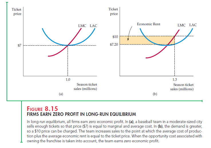
Because more people want to see baseball games, the latter team can sell tickets for $10 apiece and thereby earn an accounting profit of $2.80 above its average cost of $7.20 on each ticket. However, the rent associated with the more desirable location represents a cost to the firm—an opportunity cost—because it could sell its fran-chise to another team. As a result, the economic profit in the larger city is also zero.

Source: Pindyck Robert, Rubinfeld Daniel (2012), Microeconomics, Pearson, 8th edition.