Evaluating the Gains and Losses from Government Policies—Consumer and Producer Surplus

We saw at the end of Chapter 2 that a government-imposed price ceil- ing causes the quantity of a good demanded to rise (at the lower price, consumers want to buy more) and the quantity supplied to fall (pro- ducers are not willing to supply as much at the lower price). The result is a shortage—i.e., excess demand. Of course, those consumers who can still buy the good will be better off because they will now pay less. (Presumably, this was the objective of the policy in the first place.) But if we also take into account those who cannot obtain the good, how much better off are consumers as a whole? Might they be worse off? And if we lump consumers and produc- ers together, will their total welfare be greater or lower, and by how much? To answer questions such as these, we need a way to measure the gains and losses from government interventions and the changes in market price and quantity that such interventions cause.

Our method is to calculate the changes in consumer and producer surplus that result from an intervention. In Chapter 4, we saw that consumer surplus measures the aggregate net benefit that consumers obtain from a competitive market. In Chapter 8, we saw how producer surplus measures the aggregate net benefit to producers. Here we will see how consumer and producer surplus can be applied in practice.

1. Review of Consumer and Producer Surplus

In an unregulated, competitive market, consumers and producers buy and sell at the prevailing market price. But remember, for some consumers the value of the good exceeds this market price; they would pay more for the good if they had to. Consumer surplus is the total benefit or value that consumers receive beyond what they pay for the good.

For example, suppose the market price is $5 per unit, as in Figure 9.1. Some consumers probably value this good very highly and would pay much more than $5 for it. Consumer A, for example, would pay up to $10 for the good. However, because the market price is only $5, he enjoys a net benefit of $5—the $10 value he places on the good, less the $5 he must pay to obtain it. Consumer B values the good somewhat less highly. She would be willing to pay $7, and thus enjoys a $2 net benefit. Finally, Consumer C values the good at exactly the market price, $5. He is indifferent between buying or not buying the good, and if the market price were one cent higher, he would forgo the purchase. Consumer C, therefore, obtains no net benefit.1

For consumers in the aggregate, consumer surplus is the area between the demand curve and the market price (i.e., the yellow-shaded area in Figure 9.1). Because consumer surplus measures the total net benefit to consumers, we can mea- sure the gain or loss to consumers from a government intervention by measur- ing the resulting change in consumer surplus.

Producer surplus is the analogous measure for producers. Some producers are producing units at a cost just equal to the market price. Other units, however, could be produced for less than the market price and would still be produced and sold even if the market price were lower. Producers, therefore, enjoy a ben- efit—a surplus—from selling those units. For each unit, this surplus is the dif- ference between the market price the producer receives and the marginal cost of producing this unit.

For the market as a whole, producer surplus is the area above the supply curve up to the market price; this is the benefit that lower-cost producers enjoy by selling at the market price. In Figure 9.1, it is the green triangle. And because pro- ducer surplus measures the total net benefit to producers, we can measure the gain or loss to producers from a government intervention by measuring the resulting change in producer surplus.

2. Application of Consumer and Producer Surplus

With consumer and producer surplus, we can evaluate the welfare effects of a government intervention in the market. We can determine who gains and who loses from the intervention, and by how much. To see how this is done, let’s return to the example of price controls that we first encountered toward the end of Chapter 2. The government makes it illegal for producers to charge more than a ceiling price set below the market-clearing level. Recall that by decreasing pro- duction and increasing the quantity demanded, such a price ceiling creates a shortage (excess demand).

Figure 9.2 replicates Figure 2.24 (page 58), except that it also shows the changes in consumer and producer surplus that result from the government price-control policy. Let’s go through these changes step by step.

1. Change in Consumer Surplus: Some consumers are worse off as a result of the policy, and others are better off. The ones who are worse off are those who have been rationed out of the market because of the reduction in production and sales from Q0 to Q1. Other consumers, however, can still purchase the good (perhaps because they are in the right place at the right time or are willing to wait in line). These consumers are better off because they can buy the good at a lower price (Pmax  rather than P0). How much better off or worse off is each group? The consumers who can still buy the good enjoy an increase in consumer surplus, which is given by the blue-shaded rectangle A. This rectangle measures the reduc-tion of price in each unit times the number of units consumers are able to buy at the lower price. On the other hand, those consumers who can no longer buy the good lose surplus; their loss is given by the green-shaded triangle B. This triangle measures the value to consumers, less what they would have had to pay, that is lost because of the reduction in output from Q0  to Q1. The net change in consumer surplus is therefore A − B. In Figure 9.2, because rectangle A is larger than triangle B, we know that the net change in consumer surplus is positive.

It is important to stress that we have assumed that those consumers who are able to buy the good are the ones who value it most highly. If that were not the case—e.g., if the output Q1  were rationed randomly— the amount of lost consumer surplus would be larger than triangle B. In many cases, there is no reason to expect that those consumers who value the good most highly will be the ones who are able to buy it. As a result, the loss of consumer surplus might greatly exceed triangle B, making price controls highly inefficient.2

In addition, we have ignored the opportunity costs that arise with rationing. For example, those people who want the good might have to wait in line to obtain it. In that case, the opportunity cost of their time should be included as part of lost consumer surplus.

2. Change in Producer Surplus: With price controls, some producers (those with relatively lower costs) will stay in the market but will receive a lower price for their output, while other producers will leave the market. Both groups will lose producer surplus. Those who remain in the market and produce quantity Q1 are now receiving a lower price. They have lost the producer surplus given by rectangle A. However, total production has also dropped. The purple-shaded triangle C measures the additional loss of producer surplus for those producers who have left the market and those who have stayed in the market but are producing less. Therefore, the total change in producer surplus is −A − C. Producers clearly lose as a result of price controls.

3. Deadweight Loss: Is the loss to producers from price controls offset by the gain to consumers? No. As Figure 9.2 shows, price controls result in a net loss of total surplus, which we call a deadweight loss. Recall that the change in consumer surplus is A − B and that the change in producer surplus is −A −  C. The total change in surplus is therefore (A −  B) + (−A − C) = −B − C. We thus have a deadweight loss, which is given by the two triangles B and C in Figure 9.2. This deadweight loss is an inefficiency caused by price controls; the loss in producer surplus exceeds the gain in consumer surplus.

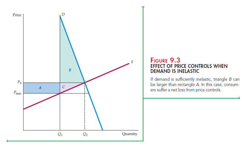
If politicians value consumer surplus more than producer surplus, this dead- weight loss from price controls may not carry much political weight. However, if the demand curve is very inelastic, price controls can result in a net loss of consumer surplus, as Figure 9.3 shows. In that figure, triangle B, which measures the loss to consumers who have been rationed out of the market, is larger than rectangle A, which measures the gain to consumers able to buy the good. Here, because consumers value the good highly, those who are rationed out suffer a large loss.

The demand for gasoline is very inelastic in the short run (but much more elastic in the long run). During the summer of 1979, gasoline shortages resulted from oil price controls that prevented domestic gasoline prices from increas- ing to rising world levels. Consumers spent hours waiting in line to buy gaso- line. This was a good example of price controls making consumers—the group whom the policy was presumably intended to protect—worse off.

Source: Pindyck Robert, Rubinfeld Daniel (2012), Microeconomics, Pearson, 8th edition.