So far, our discussions of market behavior have been largely based on partial equilibrium analysis. When determining the equilibrium prices and quantities in a market using partial equilibrium analysis, we presume that activity in one market has little or no effect on other markets. For example, in Chapters 2 and 9, we presumed that the wheat market was largely independent of the markets for related products, such as corn and soybeans.
Often a partial equilibrium analysis is sufficient to understand market behavior. However, market interrelationships can be important. In Chapter 2, for example, we saw how a change in the price of one good can affect the demand for another if they are complements or substitutes. In Chapter 8, we saw that an increase in a firm’s input demand can cause both the market price of the input and the product price to rise.
Unlike partial equilibrium analysis, general equilibrium analysis determines the prices and quantities in all markets simultaneously, and it explicitly takes feedback effects into account. A feedback effect is a price or quantity adjustment in one market caused by price and quantity adjustments in related markets. Suppose, for example, that the U.S. government taxes oil imports. This policy would immediately shift the supply curve for oil to the left (by making foreign oil more expensive) and raise the price of oil. But the effect of the tax would not end there. The higher price of oil would increase the demand for and then the price of natural gas. The higher natural gas price would in turn cause oil demand to rise (shift to the right) and increase the oil price even more. The oil and natural gas markets will continue to interact until eventually an equilibrium is reached in which the quantity demanded and quantity supplied are equated in both markets.
In practice, a complete general equilibrium analysis, which evaluates the effects of a change in one market on all other markets, is not feasible. Instead, we confine ourselves to two or three markets that are closely related. For example, when looking at a tax on oil, we might also look at markets for natural gas, coal, and electricity.
1. Two Interdependent Markets—Moving to General Equilibrium
To study the interdependence of markets, let’s examine the competitive markets for DVD rentals and movie theater tickets. The two markets are closely related because DVD players give most consumers the option of watching movies at home as well as at the theater. Changes in pricing policies that affect one market are likely to affect the other, which in turn causes feedback effects in the first market.
Figure 16.1 shows the supply and demand curves for DVDs and movies. In part (a), the price of movie tickets is initially $6.00; the market is in equilibrium at the intersection of DM and SM. In part (b), the DVD market is also in equilibrium with a price of $3.00.
Now suppose that the government places a tax of $1 on each movie ticket purchased. The effect of this tax is determined on a partial equilibrium basis by shifting the supply curve for movies upward by $1, from SM to SM in Figure 16.1 (a). Initially, this shift causes the prices of movies to increase to $6.35 and the quantity of movie tickets sold to fall from QM to QM. This is as far as a partial equilibrium analysis takes us. But we can go further with a general equilibrium analysis by doing two things: (1) looking at the effects of the movie tax on the market for DVDs, and (2) seeing whether there are any feedback effects from the DVD market to the movie market.
The movie tax affects the market for DVDs because movies and DVDs are substitutes. A higher movie price shifts the demand for DVDs from DV to D’V in Figure 16.1 (b). In turn, this shift causes the rental price of DVDs to increase from $3.00 to $3.50. Note that a tax on one product can affect the prices and sales of other products—something that policymakers should remember when designing tax policies.
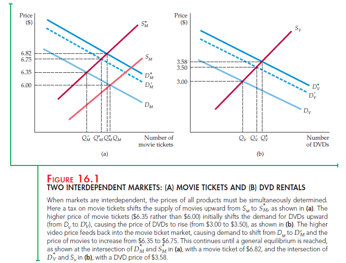
What about the market for movies? The original demand curve for movies presumed that the price of DVDs was unchanged at $3.00. But because that price is now $3.50, the demand for movies will shift upward, from DM to D ‘M in Figure 16.1 (a). The new equilibrium price of movies (at the intersection of SM and DM) is $6.75, instead of $6.35, and the quantity of movie tickets purchased has increased from QM to Q M. Thus a partial equilibrium analysis would have underestimated the effect of the tax on the price of movies. The DVD market is so closely related to the market for movies that to determine the tax’s full effect, we need a general equilibrium analysis.
2. Reaching General Equilibrium
Our analysis is not yet complete. The change in the market price of movies will generate a feedback effect on the price of DVDs that, in turn, will affect the price of movies, and so on. In the end, we must determine the equilibrium prices and quantities of both movies and DVDs simultaneously. The equilibrium movie price of $6.82 is given in Figure 16.1 (a) by the intersection of the equilibrium supply and demand curves for movie tickets (SM and D M). The equilibrium DVD price of $3.58 is given in Figure 16.1 (b) by the intersection of the equilibrium supply and demand curves for DVDs (SV and DV). These are the correct general equilibrium prices because the DVD market supply and demand curves have been drawn on the assumption that the price of movie tickets is $6.82. Likewise, the movie ticket curves have been drawn on the assumption that the price of DVDs is $3.58. In other words, both sets of curves are consistent with the prices in related markets, and we have no reason to expect that the supply and demand curves in either market will shift further. To find the general equilibrium prices (and quantities) in practice, we must simultaneously find two prices that equate quantity demanded and quantity supplied in all related markets. For our two markets, we need to find the solution to four equations (supply of movie tickets, demand for movie tickets, supply of DVDs, and demand for DVDs).
Note that even if we were only interested in the market for movies, it would be important to account for the DVD market when determining the impact of a movie tax. In this example, partial equilibrium analysis would lead us to conclude that the tax will increase the price of movie tickets from $6.00 to $6.35. A general equilibrium analysis, however, shows us that the impact of the tax on the price of movie tickets is greater: It would in fact increase to $6.82.
Movies and DVDs are substitute goods. By drawing diagrams analogous to those in Figure 16.1, you should be able to convince yourself that if the goods in question are complements, a partial equilibrium analysis will overstate the impact of a tax. Think about gasoline and automobiles, for example. A tax on gasoline will cause its price to go up, but this increase will reduce demand for automobiles, which in turn reduces the demand for gasoline, causing its price to fall somewhat.
Source: Pindyck Robert, Rubinfeld Daniel (2012), Microeconomics, Pearson, 8th edition.
I like this web site because so much useful material on here : D.
I am glad to be a visitant of this consummate blog! , thankyou for this rare information! .