The Nash Equilibrium Revisited

To determine the likely outcome of a game, we have been seeking “self-enforc- ing,” or “stable” strategies. Dominant strategies are stable, but in many games, one or more players do not have a dominant strategy. We therefore need a more general equilibrium concept. In Chapter 12, we introduced the concept of a Nash equilibrium and saw that it is widely applicable and intuitively appealing.5

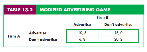
Recall that a Nash equilibrium is a set of strategies (or actions) such that each player is doing the best it can given the actions of its opponents. Because each player has no incentive to deviate from its Nash strategy, the strategies are stable. In the example shown in Table 13.2, the Nash equilibrium is that both firms advertise: Given the decision of its competitor, each firm is satisfied that it has made the best decision possible, and so has no incentive to change its decision.

In Chapter 12, we used the Nash equilibrium to study output and pricing by oligopolistic firms. In the Cournot model, for example, each firm sets its own output while taking the outputs of its competitors as fixed. We saw that in a Cournot equilibrium, no firm has an incentive to change its output unilaterally because each firm is doing the best it can given the decisions of its competitors. Thus a Cournot equilibrium is a Nash equilibrium.6  We also examined mod- els in which firms choose price, taking the prices of their competitors as fixed. Again, in the Nash equilibrium, each firm is earning the largest profit it can given the prices of its competitors, and thus has no incentive to change its price.

It is helpful to compare the concept of a Nash equilibrium with that of an equilibrium in dominant strategies:

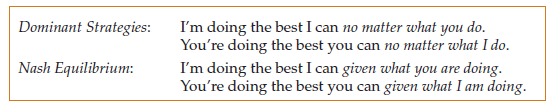
Note that a dominant strategy equilibrium is a special case of a Nash equilibrium.

In the advertising game of Table 13.2, there is a single Nash equilibrium—both firms advertise. In general, a game need not have a single Nash equilibrium. Sometimes there is no Nash equilibrium, and sometimes there are several (i.e., several sets of strategies are stable and self-enforcing). A few more examples will help to clarify this.

THE PRODUCT CHOICE PROBLEM Consider the following “product choice” problem. Two breakfast cereal companies face a market in which two new varia- tions of cereal can be successfully introduced—provided that each variation is introduced by only one firm. There is a market for a new “crispy” cereal and a market for a new “sweet” cereal, but each firm has the resources to introduce only one new product. The payoff matrix for the two firms might look like the one in Table 13.3.

In this game, each firm is indifferent about which product it produces—so long as it does not introduce the same product as its competitor. If coordina- tion were possible, the firms would probably agree to divide the market. But what if the firms must behave noncooperatively? Suppose that somehow—per- haps through a news release—Firm 1 indicates that it is about to introduce the sweet cereal, and that Firm 2 (after hearing this) announces its plan to introduce the crispy one. Given the action that it believes its opponent to be taking, nei- ther firm has an incentive to deviate from its proposed action. If it takes the proposed action, its payoff is 10, but if it deviates—and its opponent’s action remains unchanged—its payoff will be – 5. Therefore, the strategy set given by the bottom left-hand corner of the payoff matrix is stable and constitutes a Nash equilibrium: Given the strategy of its opponent, each firm is doing the best it can and has no incentive to deviate.

Note that the upper right-hand corner of the payoff matrix is also a Nash equilibrium, which might occur if Firm 1 indicated that it was about to produce the crispy cereal. Each Nash equilibrium is stable because once the strategies are chosen, no player will unilaterally deviate from them. However, without more information, we have no way of knowing which equilibrium (crispy/sweet  vs. sweet/crispy)  is likely to result—or if either will result. Of course, both firms have a strong incentive to reach one of the two Nash equilibria—if they both introduce the same type of cereal, they will both lose money. The fact that the two firms are not allowed to collude does not mean that they will not reach a Nash equilibrium. As an industry develops, understandings often evolve as firms “signal” each other about the paths the industry is to take.

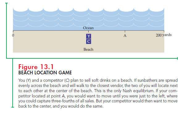
THE BEACH LOCATION GAME  Suppose that you (Y) and a competitor (C) plan to sell soft drinks on a beach this summer. The beach is 200 yards long, and sunbathers are spread evenly across its length. You and your competitor sell the same soft drinks at the same prices, so customers will walk to the closest vendor. Where on the beach will you locate, and where do you think your competitor will locate?

If you think about this for a minute, you will see that the only Nash equi- librium calls for both you and your competitor to locate at the same spot in the center of the beach (see Figure 13.1). To see why, suppose your competitor located at some other point (A), which is three quarters of the way to the end of the beach. In that case, you would no longer want to locate in the center; you would locate near your competitor, just to the left. You would thus capture nearly three-fourths of all sales, while your competitor got only the remaining fourth. This outcome is not an equilibrium because your competitor would then want to move to the center of the beach, and you would do the same.

The “beach location game” can help us understand a variety of phenom- ena. Have you ever noticed how, along a two- or three-mile stretch of road, two or three gas stations or several car dealerships will be located close to each other? Likewise, as a U.S. presidential election approaches, the Democratic and Republican candidates typically move close to the center as they define their political positions.

1. Maximin Strategies

The concept of a Nash equilibrium relies heavily on individual rationality. Each player ’s choice of strategy depends not only on its own rationality, but also on the rationality of its opponent. This can be a limitation, as the example in Table 13.4 shows.

In this game, two firms compete in selling file-encryption software. Because both firms use the same encryption standard, files encrypted by one firm’s soft- ware can be read by the other ’s—an advantage for consumers. Nonetheless, Firm 1 has a much larger market share. (It entered the market earlier and its soft- ware has a better user interface.) Both firms are now considering an investment in a new encryption standard.

Note that investing is a dominant strategy for Firm 2 because by doing so it will do better regardless of what Firm 1 does. Thus Firm 1 should expect Firm 2 to invest. In this case, Firm 1 would also do better by investing (and earning $20 million) than by not investing (and losing $10 million). Clearly the outcome (invest, invest) is a Nash equilibrium for this game, and you can verify that it is the only Nash equilibrium. But note that Firm 1’s managers had better be sure that Firm 2’s managers understand the game and are rational. If Firm 2 should happen to make a mistake and fail to invest, it would be extremely costly to Firm 1. (Consumer confusion over incompatible standards would arise, and Firm 1, with its dominant market share, would lose $100 million.)

If you were Firm 1, what would you do? If you tend to be cautious—and if you are concerned that the managers of Firm 2 might not be fully informed or rational—you might choose to play “don’t invest.” In that case, the worst that can happen is that you will lose $10 million; you no longer have a chance of los- ing $100 million. This strategy is called a maximin strategy because it maximizes the minimum gain that can be earned. If both firms used maximin strategies, the outcome would be that Firm 1 does not invest and Firm 2 does. A maximin strat- egy is conservative, but it is not profit-maximizing. (Firm 1, for example, loses

$10 million rather than earning $20 million.) Note that if Firm 1 knew for certain that Firm 2 was using a maximin strategy, it would prefer to invest (and earn $20 million) instead of following its own maximin strategy of not investing.

MAXIMIZING  THE EXPECTED PAYOFF If Firm 1 is unsure about what Firm 2 will do but can assign probabilities to each feasible action for Firm 2, it could instead use a strategy that maximizes its expected payoff. Suppose, for example, that Firm 1 thinks that there is only a 10-percent chance that Firm 2 will not invest. In that case, Firm 1’s expected payoff from investing is (.1)(-100) + (.9)(20) = $8 million. Its expected payoff if it doesn’t invest is (.1)(0) + (.9)(-10) = -$9 million. In this case, Firm 1 should invest.

On the other hand, suppose Firm 1 thinks that the probability that Firm 2 will not invest is 30 percent. Then Firm 1’s expected payoff from investing is (.3) (-100) + (.7)(20) = -$16 million, while its expected payoff from not investing is (.3)(0) + (.7)(-10) = -$7 million. Thus Firm 1 will choose not to invest.

You can see that Firm 1’s strategy depends critically on its assessment of the probabilities of different actions by Firm 2. Determining these probabilities may seem like a tall order. However, firms often face uncertainty (over market con- ditions, future costs, and the behavior of competitors), and must make the best decisions they can based on probability assessments and expected values.

THE PRISONERS’ DILEMMA  What is the Nash equilibrium for the prisoners’ dilemma discussed in Chapter 12? Table 13.5 shows the payoff matrix for the prisoners’ dilemma. Recall that the ideal outcome is one in which neither pris- oner confesses, so that both get two years in prison. Confessing, however, is a dominant strategy for each prisoner—it yields a higher payoff regardless of the strategy of the other prisoner. Dominant strategies are also maximin strategies.

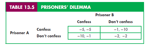
Therefore, the outcome in which both prisoners confess is both a Nash equilib- rium and a maximin solution. Thus, in a very strong sense, it is rational for each prisoner to confess.

2. Mixed Strategies

In all of the games that we have examined so far, we have considered strategies in which players make a specific choice or take a specific action: advertise or don’t advertise, set a price of $4 or a price of $6, and so on. Strategies of this kind are called pure strategies. There are games, however, in which a pure strategy is not the best way to play.

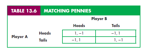
MATCHING  PENNIES An example is the game of “Matching Pennies.” In this game, each player chooses heads or tails and the two players reveal their coins at the same time. If the coins match (i.e., both are heads or both are tails), Player A wins and receives a dollar from Player B. If the coins do not match, Player B wins and receives a dollar from Player A. The payoff matrix is shown in Table 13.6.

Note that there is no Nash equilibrium in pure strategies for this game. Suppose, for example, that Player A chose the strategy of playing heads. Then Player B would want to play tails. But if Player B plays tails, Player A would also want to play tails. No combination of heads or tails leaves both players sat- isfied—one player or the other will always want to change strategies.

Although there is no Nash equilibrium in pure strategies, there is a Nash equilibrium in mixed strategies: strategies in which players make random choices among two or more possible actions, based on sets of chosen probabilities. In this game, for example, Player A might simply flip the coin, thereby playing heads with probability 1/2  and playing tails with probability 1/2.  In fact, if Player A fol- lows this strategy and Player B does the same, we will have a Nash equilib- rium: Both players will be doing the best they can given what the opponent is doing. Note that although the outcome is random, the expected payoff is 0 for each player.

It may seem strange to play a game by choosing actions randomly. But put yourself in the position of Player A and think what would happen if you followed a strategy other than just flipping the coin. Suppose you decided to play heads. If Player B knows this, she would play tails and you would lose. Even if Player B didn’t know your strategy, if the game were played repeatedly, she could even- tually discern your pattern of play and choose a strategy that countered it. Of course, you would then want to change your strategy—which is why this would not be a Nash equilibrium. Only if you and your opponent both choose heads or tails randomly with probability 1/2  would neither of you have any incentive to change strategies. (You can check that the use of different probabilities, say 3/4 for heads and 1/4  for tails, does not generate a Nash equilibrium.)

One reason to consider mixed strategies is that some games (such as “Matching Pennies”) do not have any Nash equilibria in pure strategies. It can be shown, however, that once we allow for mixed strategies, every game has at least one Nash equilibrium.7  Mixed strategies, therefore, provide solutions to games when pure strategies fail. Of course, whether solutions involving mixed strategies are reasonable will depend on the particular game and players. Mixed strategies are likely to be very reasonable for “Matching Pennies,” poker, and other such games. A firm, on the other hand, might not find it reasonable to believe that its competitor will set its price randomly.

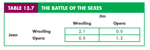
THE BATTLE OF THE SEXES Some games have Nash equilibria both in pure strategies and in mixed strategies. An example is “The Battle of the Sexes,” a game that you might find familiar. It goes like this. Jim and Joan would like to spend Saturday night together but have different tastes in entertainment. Jim would like to go to the opera, but Joan prefers mud wrestling. As the payoff matrix in Table 13.7 shows, Jim would most prefer to go to the opera with Joan, but prefers watching mud wrestling with Joan to going to the opera alone, and similarly for Joan.

First, note that there are two Nash equilibria in pure strategies for this game— the one in which Jim and Joan both watch mud wrestling, and the one in which they both go to the opera. Joan, of course, would prefer the first of these out- comes and Jim the second, but both outcomes are equilibria—neither Jim nor Joan would want to change his or her decision, given the decision of the other.

This game also has an equilibrium in mixed strategies: Joan chooses wres- tling with probability 2/3  and opera with probability 1/3,  and Jim chooses wrestling with probability 1/3  and opera with probability 2/3.  You can check that if Joan uses this strategy, Joan cannot do better with any other strategy, and vice versa.8  The outcome is random, and Jim and Joan will each have an expected payoff of 2/3.

Should we expect Jim and Joan to use these mixed strategies? Unless they’re very risk loving or in some other way a strange couple, probably not. By agreeing to either form of entertainment, each will have a payoff of at least as in many others, mixed strategies provide another solution, but not a very realistic one. Hence, for the remainder of this chapter we will focus on pure strategies.

Source: Pindyck Robert, Rubinfeld Daniel (2012), Microeconomics, Pearson, 8th edition.