Cluster Analysis — 2

Discovering a simple, robust typology to describe nine planets was straightforward. For a more challenging example, consider the cross-national data in Nations2.dta. These United Nations human-development variables could be applied to develop an empirical typology of nations.

. use C:\data\Natlons2.dta, clear

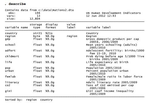
Working with the same data in Chapter7, we saw that nonlinear transformations such as logarithms helped to normalize distributions and linearize relationships among some of these variables. Similar arguments for nonlinear transformations could apply to cluster analysis, but to keep the example simple they are not pursued here. Linear transformations to standardize the variables in some fashion remain essential, however. Otherwise, the variable gdp, which ranges from about $280 to $74,906 (standard deviation $13,942) would overwhelm other variables such as life, which ranges from about 46 to 83 years (standard deviation 10 years). In the previous section, we standardized planetary data by subtracting each variable’s mean, then dividing by its standard deviation, so that the resulting z-scores all had standard deviations of one. In this section we take a different approach, range standardization, which also works well for cluster analysis.

Range standardization involves dividing each variable by its range. There is no command to do this directly in Stata, but we can improvise one easily enough. To do so, we make use of results that Stata stores unobtrusively after summarize. Recall that we can see a complete list of stored results after summarize by typing the command return list. (After modeling procedures such as regress or factor, use the command ereturn list instead.) In this example, we view the results stored after summarize pop, then use the maximum and minimum values (stored as scalars that Stata calls r(max) and r(min)) to calculate a new, range-standardized version of population.

Similar commands create range-standardized versions of other living-conditions variables:

. quietly summ school

. generate rschool = school/(r(max) – r(min))

. label variable rschool “Range-standardized schooling”

. quietly summ adfert

. generate radfert = adfert/(r(max) – r(min))

. label variable radfert “Range-standardized adolescent fertility”

and so forth, defining the 8 new variables listed below.

If our generate commands were done correctly, these new range-standardized variables should all have ranges equal to 1. tabstat confirms that they do.

Once the variables of interest have been standardized, we can proceed with cluster analysis. As we divide more than 100 nations into types, we have no reason to assume that each type will include a similar number of nations. Average linkage (used in our planetary example), along
with some other methods, gives each observation the same weight. This tends to make larger clusters more influential as agglomeration proceeds. Weighted average and median linkage methods, on the other hand, give equal weight to each cluster regardless of how many observations it contains. Such methods consequently tend to work better for detecting clusters of unequal size. Median linkage, like centroid linkage, is subject to reversals (which will occur with these data), so the following example applies weighted average linkage. Absolute-value distance (measure(Ll)) provides our dissimilarity measure.

. cluster waveragelinkage rgdp – rfemlab, measure(Ll) name(Llwav)

The full cluster analysis proves unmanageably large for a dendrogram:

Following the error-message advice, Figure 11.5 employs a cutnumber(100) option to form a dendrogram that starts with only 100 groups, after the first few fusions have taken place.

The bottom labels in Figure 11.5 are unreadable, but we can trace the general flow of this clustering process. Most of the fusion takes place at dissimilarities below 1. Two nations just right of center in the dendrogram are unusual; they resist fusion until about 2 and then form a stable two-nation group quite different from all the rest. This is one of four clusters remaining at dissimilarities above 2. The first and fourth of these four final clusters (reading left to right) appear heterogeneous, formed through successive fusion of a number of somewhat distinct major subgroups. The second cluster, in contrast, appears more homogeneous. It combines many nations that fused into two subgroups at dissimilarities below 1, and then fused into one group at slightly above 1.

Figure 11.6 gives another view of this analysis, this time using the cutvalue(1.2) option to show only clusters with dissimilarities above 1.2, after most of the fusions have taken place. The showcount option calls for bottom labels ( n=13, n=11, etc.) that indicate the number of nations in each group. We see that groups 8, 9 and 12 each consists of a single nation.

As Figure 11.6 shows, there are 15 groups remaining at dissimilarities above 1.2. For purposes of illustration, we will consider only the top four groups, which have dissimilarities above 2. cluster generate creates a categorical variable for the final four groups from the cluster analysis we named Llwav.

. cluster generate ctype = groups(4), name(Llwav)

. label variable ctype “Country type”

We could next examine which countries belong to which groups by typing

. sort cype

. by ctype: list country

The long list that results is not shown here, but it reveals that the two-nation cluster we noticed in Figure 11.5 is type 3, India and China. The relatively homogeneous second cluster in Figure 11.5, now classified as type 4, contains a large group of the poorest nations, mainly in Africa. The relatively diverse type 2 contains more affluent nations including the U.S., Japan and many in Europe. Type 1, also diverse, contains nations with intermediate living conditions. Whether this or some other typology is meaningful remains a substantive question, not a statistical one, and depends on the uses for which the typology is needed. Choosing different options in the steps of our cluster analysis would have returned different results. By experimenting with a variety of reasonable choices, we could gain a sense of which findings are most stable.

Source: Hamilton Lawrence C. (2012), Statistics with STATA: Version 12, Cengage Learning; 8th edition.