Cluster Analysis — 1

Cluster analysis encompasses a variety of methods that divide observations into groups or clusters, based on their dissimilarities across a number of variables. It is most often used as an exploratory approach, for developing empirical typologies, rather than as a means of testing pre­specified hypotheses. Indeed, there exists little formal theory to guide hypothesis testing for the common clustering methods. The number of choices available at each step in the analysis is daunting, and all the more so because they can lead to many different results. This section provides an entry point to beginning cluster analysis. We review some basic ideas and illustrate them through a simple example. The section that follows considers a somewhat larger example. Stata’s Multivariate Statistics Reference Manual introduces and defines the full range of choices available. Everitt etal. (2001) cover topics in more detail, including helpful comparisons among the many cluster-analysis methods.

All clustering methods begin with some definition of dissimilarity (or similarity). Dissimilarity measures reflect the differentness or distance between two observations, across a specified set of variables. Generally, such measures are designed so that two identical observations have a dissimilarity of 0, and two maximally different observations have a dissimilarity of 1. Similarity measures reverse this scaling, so that identical observations have a similarity of 1. Stata’s cluster options offer many choices of dissimilarity or similarity measures. For purposes of calculation, Stata internally transforms similarity to dissimilarity:

dissimilarity = 1 – similarity

The default dissimilarity measure for averagelinkage, completelinkage, singlelinkage and waveragelinkage is the Euclidean distance, option measure(L2). This defines the distance between observations i and j as

where x _ki is the value of variable x _k for observation i, x _kj the value of x _k for observation j, and summation occurs over all the x variables considered. Other choices available for measuring the (dis)similarities between observations based on continuous variables include the squared Euclidean distance (L2squared, default for centroidlinkage, medianlinkage and wardslinkage), the absolute-value distance (L1), maximum-value distance (Linfinity) and correlation coefficient similarity measure (correlation). Choices for binary variables include simple matching (matching), Jaccard binary similarity coefficient (Jaccard) and others. The gower option works with a mix of continuous and binary variables. Type help measure option for a complete list and detailed explanations of dissimilarity-measure options.

Clustering methods fall into two broad categories,partition and hierarchical. Partition methods break the observations into a pre-set number of nonoverlapping groups. We have two ways to do this:

cluster kmeans        Kmeans cluster analysis

User specifies the number of clusters (K) to create. Stata then finds these through an iterative process, assigning observations to the group with the closest mean.

cluster kmedians       Kmedians cluster analysis Similar to

Kmeans, but with medians.

Partition methods tend to be computationally simpler and faster than hierarchical methods. The necessity of declaring the exact number of clusters in advance is a disadvantage for exploratory work, however.

Hierarchical methods involve a process of small groups gradually fusing to form increasingly large ones. Stata takes an agglomerative approach in hierarchical cluster analysis: It starts out with each observation considered as its own separate group. The closest two groups are merged, and this process continues until a specified stopping-point is reached, or all observations belong to one group. A graphical display called a dendrogram or tree diagram visualizes hierarchical clustering results. Several choices exist for the linkage method, which specifies what should be compared between groups that contain more than one observation:

cluster singlelinkage         Single linkage cluster analysis

Computes the dissimilarity between two groups as the dissimilarity between the least different pair of observations in the two groups. Although simple, this method has low resistance to outliers or measurement errors. Observations tend to join clusters one at a time, forming unbalanced, drawn-out groups in which members have little in common, but are linked by intermediate observations — a problem called chaining.

cluster averagelinkage        Average linkage cluster analysis

Uses the average dissimilarity of observations in the two groups, yielding properties intermediate between single and complete linkage. Simulation studies report that this works well for many situations and is reasonably robust (see Everitt et al. 2001, and sources they cite). Commonly used in archaeology.

cluster completelinkage        Complete linkage cluster analysis

Uses the least similar pair of observations in the two groups. Less sensitive to outliers than single linkage, but with the opposite tendency towards clumping many observations into tight, spatially compact clusters.

cluster waveragelinkage        Weighted-average linkage cluster analysis

cluster medianlinkage            Median linkage cluster analysis.

Weighted-average linkage and median linkage are variations on average linkage and centroid linkage, respectively. In both cases, the difference is in how groups of unequal size are treated when merged. In average linkage and centroid linkage, the number of elements of each group are factored into the computation, giving correspondingly larger influence to the larger group (because each observation carries the same weight). In weighted-average linkage and median linkage, the two groups are given equal weighting regardless of how many observations there are in each group. Median linkage, like centroid linkage, is subject to reversals.

cluster centroidlinkage            Centroid linkage cluster analysis

Centroid linkage merges the groups whose means are closest (in contrast to average linkage which looks at the average distance between elements of the two groups). This method is subject to reversals — points where a fusion takes place at a lower level of dissimilarity than an earlier fusion. Reversals signal an unstable cluster structure, are difficult to interpret, and cannot be graphed by cluster dendrogram.

cluster wardslinkage            Ward’s linkage cluster analysis

Joins the two groups that result in the minimum increase in the error sum of squares. Does well with groups that are multivariate normal and of similar size, but poorly when clusters have unequal numbers of observations.

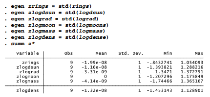
Earlier in this chapter, a principal component factor analysis of variables inplanets.dta (Figure 11.3) identified three types of planets: inner rocky planets, outer gas giants and, in a class by itself, Pluto. Cluster analysis provides an alternative approach to the question of planet types. Because variables such as number of moons (moons) and mass in kilograms (mass) are measured in incomparable units, with hugely different variances, we should standardize in some way to avoid results dominated by the highest-variance items. A common, although not automatic, choice is standardization to zero mean and unit standard deviation. This is accomplished through the egen command (and using variables in log form, for the same reasons discussed earlier). summarize confirms that the new z variables have (near) zero means, and standard deviations equal to one.

The “three types” conclusion suggested by our principal component factor analysis is robust, and could have been found through cluster analysis as well. For example, we might perform a hierarchical cluster analysis with average linkage, using Euclidean distance (L2) as our dissimilarity measure. The option name(L2avg) gives the results from this particular analysis a name, so that we can refer to them in later commands. The results-naming feature is convenient when we need to try a number of cluster analyses and compare their outcomes.

. cluster averagelinkage zrings zlogdsun zlograd zlogmoon zlogmass zlogdens, measure(L2) name(L2avg)

Nothing seems to happen, although we might notice that our dataset now contains three new variables with names based on L2avg. These new L2avg* variables are not directly of interest, but can be used unobtrusively by the cluster dendrogram command to draw a cluster analysis tree or dendrogram visualizing the most recent hierarchical cluster analysis results (Figure 11.4). The label(planet) option here causes planet names (values ofplanet) to appear as labels below the graph.

Dendrograms such as Figure 11.4 provide key interpretive tools for hierarchical cluster analysis. We can trace the agglomerative process from each observation comprising its own unique cluster, at bottom, to all fused into one cluster, at top. Venus and Earth, and also Uranus and Neptune, are the least dissimilar or most alike pairs. They are fused first, forming the first two multi-observation clusters at a height (dissimilarity) below 1. Jupiter and Saturn, then Venus-Earth and Mars, then Venus-Earth-Mars and Mercury, and finally Jupiter-Saturn and Uranus-Neptune are fused in quick succession, all with dissimilarities slightly above 1. At this point we have the same three groups suggested in Figure 11.3 by principal components: the inner rocky planets, the gas giants and Pluto. The three clusters remain stable until, at much higher dissimilarity (above 3), Pluto fuses with the inner rocky planets. At a dissimilarity above 4, the final two clusters fuse.

So, how many types of planets are there? Figure 11.4 makes clear that the answer is “it depends.” How much dissimilarity do we want to accept within each type? The long vertical lines between the three-cluster stage and the two-cluster stage in the upper part of the graph indicate that we have three fairly distinct types. We could reduce this to two types only by fusing an observation (Pluto) that is quite dissimilar to others in its group. We could expand it to five types only by drawing distinctions between several planets (e.g., Mercury and Venus-Earth-Mars) that by solar-system standards are not greatly dissimilar. Thus, the dendrogram makes a case for a three-type scheme.

The cluster generate command creates a new variable indicating the type or group to which each observation belongs. In this example, groups(3) calls for three groups. The name(L2avg) option specifies the particular results we named L2avg. This option is most useful when our session included multiple cluster analyses.

The inner rocky planets have been coded as plantype = 1, the gas giants as plantype = 3, and Pluto is by itself as plantype = 2. The group designations as 1, 2 and 3 follow the left-to-right ordering of final clusters in the dendrogram (Figure 11.4). Once the data have been saved, our new typology could be used like any other categorical variable in subsequent analyses.

These planetary data have a strong pattern of natural groups, which is why such different techniques as cluster analysis and principal components point towards similar conclusions. We could have chosen other dissimilarity measures and linkage methods for this example, and still arrived at much the same place. Complex or weakly patterned data, on the other hand, often yield quite different results depending on the methods used. The clusters found by one method might not prove replicable under other methods, or with slightly different analytical decisions.

Source: Hamilton Lawrence C. (2012), Statistics with STATA: Version 12, Cengage Learning; 8th edition.