Correlation in Linear Regression by using Stata

Ordinary least-squares (OLS) regression finds the best-fitting straight line. A Pearson product- moment correlation coefficient describes how well the best-fitting line fits. correlate obtains correlations for listed variables.

. correlate gdp school adfert chldmort life

correlate reports correlations based only on those observations that have non-missing values on all of the listed variables. From the table above we learn that only 178 of the 194 nations in Nations2.dta have complete information on all five of these variables. Those 178 correspond to the subset of observations that would be used in fitting models such as a multiple regression analysis that involves all of these variables.

Analysts not employing regression or other multi-variable techniques, however, might prefer to find correlations based on all of the observations available for each variable pair. The command pwcorr (pairwise correlation) accomplishes this. It can also furnish f-test probabilities for the null hypotheses that each individual correlation equals zero. In this example, the star(.05) option requests stars (*) marking correlations individually significant at the a = .05 level.

It is worth recalling, however, that if we drew many random samples from a population in which all variables really had zero correlations, about 5% of the sample correlations would nonetheless test “statistically significant” at the .05 level. Inexperienced analysts who review many individual hypothesis tests such as those in a pwcorr matrix, to identify the handful that are significant at the .05 level, run a much higher than .05 risk of making a Type I error. This problem is called the multiple-comparison fallacy. pwcorr offers two methods, Bonferroni and Sidak, for adjusting significance levels to take multiple comparisons into account. Of these, the Sidak method is more accurate. Significance-test probabilities are adjusted for the number of comparisons made.

. pwcorr gdp school adfert chldmort life, sidak sig star(.05)

The adjustments have minor effects with the moderate to strong correlations above, but could become critical with weaker correlations or more variables. In general, the more variables we correlate, the more the adjusted probabilities will exceed their unadjusted counterparts. See the Base Reference Manual’s discussion of oneway for the formulas involved.

Because Pearson correlations measure how well an OLS regression line fits, such correlations share the assumptions and weaknesses of OLS. Like OLS, correlations should generally not be interpreted without a look at the corresponding scatterplots. Scatterplot matrices provide a quick way to do this, using the same organization as a correlation matrix. Figure 3.12 in Chapter 3 shows a scatterplot matrix corresponding to the pwcorr commands above. By default, graph matrix applies pairwise deletion like pwcorr, so each small scatterplot shows all observations with nonmissing values on that particular pair of variables.

To obtain a scatterplot matrix corresponding to a correlate matrix or multiple regression, from which all observations having missing values are omitted, we qualify the command. One way to exclude observations with missing values on any of the listed variables employs the “not missing” (!missing) function (Figure 7.3):

. graph matrix gdp school adfert chldmort life

if lmissing(gdp,school,adfert,chldmort,life), half msymbol(+)

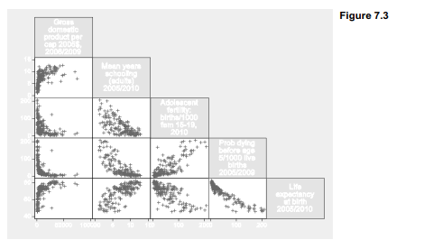
Figure 7.3 reveals what the correlation matrix does not: relationships involving per capita GDP are distinctly nonlinear. Consequently the correlation coefficients, or linear regression, provide poor descriptions of these relationships, and their significance tests are invalid.

Adding the covariance option after correlate produces a matrix of variances and covariances instead of correlations.

. correlate w x y z, covariance

Typing the following after a regression analysis displays the matrix of correlations between estimated coefficients, sometimes used to diagnose multicollinearity.

. estat vce, correlation

The following command will display the estimated coefficients’ variance-covariance matrix, from which standard errors are derived.

. estat vce

In addition to Pearson correlations, Stata can also calculate several rank-based correlations. These can be employed to measure associations between ordinal variables, or as an outlier- resistant alternative to Pearson correlation for measurement variables. To obtain the Spearman rank correlation between life and school, equivalent to the Pearson correlation if these variables were transformed into ranks, type

. spearman life school

Number of obs =  188

Spearman’s rho =   0.7145

lest of Ho:     life and school are independent

Prob > |t| =   0.0000

Kendall’s T_a (tau-a) and T_b (tau-b) rank correlations can be found easily for these data, although with larger datasets their calculation becomes slow:

For comparison, here is the Pearson correlation with its unadjusted p-value:

In this example, both spearman (.71) and pwcorr (.73) yield higher correlations than ktau (.51). All three agree that null hypotheses of no association can be rejected.

Source: Hamilton Lawrence C. (2012), Statistics with STATA: Version 12, Cengage Learning; 8th edition.