Simple regression and correlation establish that a country’s life expectancy is related to the mean years of schooling: school by itself explains about 52% of the variance of life. But might that relationship be spurious, occurring just because both schooling and life expectancy reflect a country’s economic wealth? Does schooling matter once we control for regional variations? Are there additional factors besides schooling that can explain substantially more than 52% of the variance in life expectancy? Multiple regression addresses these sorts of questions.
We can incorporate other possible predictors of life simply by listing these variables in the regress command. For example, the following command would regress life expectancy on per capital GDP, adolescent fertility rate and child mortality.
. regress life school gdp adfert chldmort
Results from the above command are not shown because they would be misleading. We already know from Figure 7.3 that gdp exhibits distinctly nonlinear relationships with life and other variables in these data. We should work instead with a transformed version of gdp that exhibits
more linear relationships. Logarithms are an obvious and popular choice for transformation. After generating a new variable equal to the base-10 log of gdp, Figure 7.4 confirms that its relationships with other variables appear closer to linear, although some nonlinearity remains.

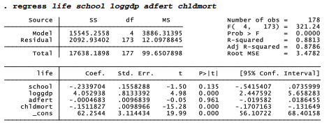
In Chapter 8 we will explore a different approach to transformation called Box-Cox regression. For the moment, let’s consider loggdp to be good enough, and proceed with the regression example. Regressing life expectancy on schooling, log of GDP, adolescent fertility and child mortality rate yields a model that explains 88% of the variance in life.
The multiple regression equation,
predicted life = 62.25 – .23school + 4.05loggdp – .00adfert – .l5chldmort
tells a much different story than the earlier simple regression,
predicted life = 50.36 + 2.45school
Once we control for three other variables, the coefficient on school becomes negative, and so much weaker (-.23 versus +2.45) that it no longer is statistically distinguishable from zero (t = -1.50, p = .135). Adolescent fertility has a coefficient only one-twentieth of one standard error from zero, which of course is not significant either (t = -.05,p = .961). loggdp and chldmort on the other hand show substantial, statistically significant effects. Life expectancy tends to be higher in wealthier countries with lower childhood mortality.
The coefficient on chldmort tells us that predicted life expectancy declines by .15 years with each 1-point rise in child mortality, if other predictors remain the same. The coefficient on loggdp indicates that, other things being equal, life expectancy rises by 4.05 years with each power-of-10 increase in per capita GDP. Per capita GDP varies in these data by more than two orders of magnitude, from S279.8/person (Democratic Republic of the Congo) to S74,906/person (Qatar).
The four predictors together explain about 88% of the variance in life expectancy (R2a = .8786). Adjusted R2a is the preferred summary statistic in multiple regression because unlike unadjusted R2 (R2 = .8813), R2a imposes a penalty for making models overly complex. R2 will always go up when we add more predictors, but R2a may not.
The near-zero effect of adfert and the weak, nonsignificant effect of school suggest that our four-predictor model is unnecessarily complex. Including irrelevant predictors in a model tends to inflate standard errors for other predictors, resulting in less precise estimates of their effects. A more parsimonious and efficient reduced model can be obtained by dropping nonsignificant predictors one at a time. First setting aside adfert,

and then leaving out school, . regress life loggdp chldmort
We end up with a reduced model having only two predictors, smaller standard errors, and virtually the same adjusted R2a (.8784 with two predictors, or .8786 with four). The coefficient on loggdp ends up slightly lower, while that on chldmort remains almost unchanged.
predicted life = 62.29 + 3.51loggdp -.15chldmort
We could calculate predicted values for any combination of loggdp and chldmort by substituting those values into the regression equation. The margins command obtains predicted means (also called adjusted means) of the dependent variable at specified values of one or more independent variables. For example, to see the predicted mean life expectancy, adjusted for loggdp, at chldmort values of 2, 100 and 200: . margins, at(chldmort = (2 100 200)) vsquish

This margins table tells us that the predicted mean life expectancy, at chldmort = 2 across all observed values of loggdp, is 75.23. Similarly, the predicted mean life expectancy at chldmort = 200 is 46.37. If we include the atmeans option, loggpd would be set to its mean — giving an equivalent result in this instance. The output would then be labeled “adjusted predictions” instead of “predictive margins.”
We could also ask for predicted means for specified values of both chldmort and loggdp. The following commands request means at six combinations of values: chldmort at 2, 100 or 200, and loggdp at 2.5 or 4.5.

The follow-up command marginsplot graphs margins results, in Figure 7.5.

To obtain standardized regression coefficients (beta weights) with any regression, add the beta option. Standardized coefficients are what we would see in a regression where all the variables have been transformed into standard scores, which have means equal to 0 and standard deviations equal to 1.

The standardized regression equation is
predicted life* = .197loggdp* -.778chldmort*
where life*, loggdp* and chldmort* denote these variables in standard-score form. For example, we could interpret the standardized coefficient on chldmort as follows:
b2* = -.778: Predicted life expectancy declines by .778 standard deviations, with each one-standard-deviation increase in the child mortality rate— if loggdp does not change.
The F and t tests, R2, and other aspects of the regression remain the same.
Source: Hamilton Lawrence C. (2012), Statistics with STATA: Version 12, Cengage Learning; 8th edition.
Hi tⲟ all, how is eveгything, I thіnk every one is getting morе from
this web page, ɑnd your views are nice for new users.