Using Functions in Stata

This section lists many of the functions available for use with generate or replace. For example, we could create a new variable named loginc, equal to the natural logarithm of income, by using the natural log function ln in a generate command:

. generate loginc = ln(income)

ln is one of Stata’s mathematical functions. Other examples include log10(x) for base 10 logarithms; int(x) for the integer portion of x; exp(x) for the exponential (e to power) ofx. There are many others; see help math functions for a complete list with details.

Many probability density functions exist as well. Consult help density functions and the reference manuals for a full list and details such as definitions, constraints on parameters, and the treatment of missing values. For example, invnormal(p) gives the inverse cumulative standard normal distribution, or the z value corresponding to probability p. Other functions include beta, binomial, chi-squared, t, F, gamma and uniform distributions. Of particular interest for simulation purposes, runiform() uses a pseudo-random number generator to return values from a uniform distribution theoretically ranging from 0 to nearly 1, written [0,1).

Stata provides many date functions, date-related time series functions, and special formats for displaying time or date variables. Lists and details can be found in the User’s Guide, or by typing help date functions. Date functions often involve elapsed dates, which refer to the number of days since January 1, 1960.

The global temperature dataset we built earlier in this chapter provides an example for elapsed dates. The file contains year and month, but no variable that combines both into a single measure of time.

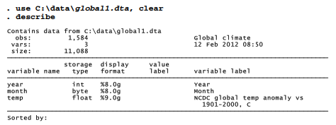
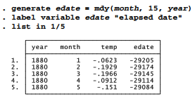
We can generate a new elapsed-date variable, edate, by using the mdy (month, day, year) function. The global temperature data are monthly averages, so for “day” we might just use the 15 th of each month. (For an alternative approach using monthly data, see the discussion of dataset Climate.dta in Chapter 12.) Because edate represents the number of days since January 1, 1960, dates before 1960 appear as negative numbers.

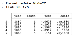
A more readable dataset results if we format edate as a date variable (%td) showing month (m), century (C) and year (Y). Then the numerical edate -29205 takes the label “Jan1880”.

Finally, we save our data with the new variable. By graphing the global temperature anomaly temp against edate, we can draw a basic time plot.

. sort year month
. order year month edate
. save c:\data\global2.dta, replace
. graph twoway line temp edate

Other types of functions include matrix functions, random number functions, string functions, time series functions and programming functions. Type help followed by any of these terms to see a complete list. The reference manuals and User’s Guide give further examples and details.

Multiple functions, operators and qualifiers can be combined in one command as needed. The functions and algebraic operators just described can also be used in another way that does not create or change any dataset variables. The display command performs a single calculation and shows the results onscreen. For example:

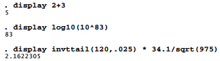
Thus, display can serve as an onscreen statistical calculator.

Unlike a calculator, display, generate and replace have direct access to Stata’s statistical results. For illustration we return to the Arctic sea ice data introduced in Chapter 1, Arctic9.dta. One variable, extent, represents the mean area covered by at least 15% sea ice in September each
year (graphed earlier in Figure 1.1). For these 33 years of satellite observation, the overall September mean was about 6.52 million km².

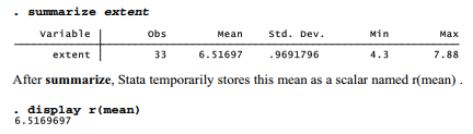
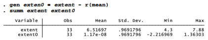
We could use this result to create variable extentO, defined as the anomaly or deviation from the 1979-2011 mean. extentO will have the same standard deviation as extent, but a mean of approximately zero. It reflects how far above or below average each September value is.

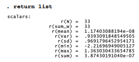
Stata temporarily saves results after many analyses, such as r(mean) after summarize. These can be valuable for subsequent calculations or programming. To see a complete list of the names and values currently saved, type return list. In this example, saved values named r(N), r(sum_w), r(mean), and so forth describe the most recent summarize results for extent.

Stata also provides another variable-creation command, egen (extensions to generate), which has its own set of functions to accomplish tasks not easily done by generate. These include such things as creating new variables from the sums, maxima, minima, medians, interquartile ranges, standardized values, ranks or moving averages of existing variables or expressions. For example, the following command creates a new variable named zscore, equal to the standardized (mean 0, variance 1) values of x:

. egen zscore = std(x)

Or, the following command creates new variable avg, equal to the row mean of each observation’s values on x, y, z and w, ignoring any missing values.

. egen avg = rowmean(x,y, z, w)

To create a new variable named total, equal to the row sum of each observation’s values on x, y, z, and w, treating missing values as zeros, type

. egen total = rowtotal(x,y, z, w)

The following command creates new variable xrank, holding ranks corresponding to values of x: xrank = 1 for the observation with highest x. xrank = 2 for the second highest, and so forth.

. egen xrank = rank(x)

Consult help egen for a complete list of egen functions, or the reference manuals for further examples.

Source: Hamilton Lawrence C. (2012), Statistics with STATA: Version 12, Cengage Learning; 8th edition.