Cost in the Short Run

In this section we focus our attention on short-run costs. We turn to long-run costs in Section 7.3.

1. The Determinants of Short-Run Cost

The data in Table 7.1 show how variable and total costs increase with output in the short run. The rate at which these costs increase depends on the nature of the production process and, in particular, on the extent to which production involves diminishing marginal returns to variable factors. Recall from Chapter 6 that diminishing marginal returns to labor occur when the marginal product of labor is decreasing. If labor is the only input, what happens as we increase the firm’s output? To produce more output, the firm must hire more labor. Then, if the marginal product of labor decreases as the amount of labor hired is increased (owing to diminishing returns), successively greater expenditures must be made to produce output at the higher rate. As a result, variable and total costs increase as the rate of output is increased. On the other hand, if the marginal product of labor decreases only slightly as the amount of labor is increased, costs will not rise so quickly when the rate of output is increased.2

Let’s look at the relationship between production and cost in more detail by concentrating on the costs of a firm that can hire as much labor as it wishes at a fixed wage w. Recall that marginal cost MC is the change in variable cost for a 1-unit change in output (i.e., AVC/Aq). But the change in variable cost is the per­unit cost of the extra labor w times the amount of extra labor needed to produce the extra output AL. Because AVC = wAL, it follows that

Recall from Chapter 6 that the marginal product of labor MP_L is the change in out­. put resulting from a 1-unit change in labor input, or Aq/AL. Therefore, the extra labor needed to obtain an extra unit of output is AL/Aq = 1/MP_L. As a result,

Equation (7.1) states that when there is only one variable input, the marginal cost is equal to the price of the input divided by its marginal product. Suppose, for example, that the marginal product of labor is 3 and the wage rate is $30 per hour. In that case, 1 hour of labor will increase output by 3 units, so that 1 unit of output will require 1/3  additional hour of labor and will cost $10. The mar- ginal cost of producing that unit of output is $10, which is equal to the wage,

$30, divided by the marginal product of labor, 3. A low marginal product of labor means that a large amount of additional labor is needed to produce more output—a fact that leads, in turn, to a high marginal cost. Conversely, a high marginal product means that the labor requirement is low, as is the marginal cost. More generally, whenever the marginal product of labor decreases, the marginal cost of production increases, and vice versa.3

DIMINISHING  MARGINAL RETURNS AND  MARGINAL COST Diminishing marginal returns means that the marginal product of labor declines as the quantity of labor employed increases. As a result, when there are diminishing marginal returns, marginal cost will increase as output increases. This can be seen by looking at the numbers for marginal cost in Table 7.1. For output levels from 0 through 4, marginal cost is declining; for output levels from 4 through 11, however, marginal cost is increasing—a reflection of the presence of diminishing marginal returns.

2. The Shapes of the Cost Curves

Figure 7.1 illustrates how various cost measures change as output changes. The top part of the figure shows total cost and its two components, variable cost and fixed cost; the bottom part shows marginal cost and average costs. These cost curves, which are based on the information in Table 7.1, provide different kinds of information.

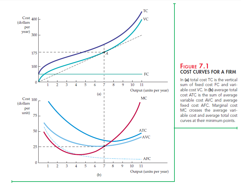
Observe in Figure 7.1 (a) that fixed cost FC does not vary with output—it is shown as a horizontal line at $50. Variable cost VC is zero when output is zero and then increases continuously as output increases. The total cost curve TC is deter- mined by vertically adding the fixed cost curve to the variable cost curve. Because fixed cost is constant, the vertical distance between the two curves is always $50.

Figure 7.1 (b) shows the corresponding set of marginal and average variable cost curves.4  Because total fixed cost is $50, the average fixed cost curve AFC falls continuously from $50 when output is 1, toward zero for large output. The shapes of the remaining curves are determined by the relationship between the marginal and average cost curves. Whenever marginal cost lies below average cost, the average cost curve falls. Whenever marginal cost lies above average cost, the average cost curve rises. When average cost is at a minimum, marginal cost equals average cost.

THE AVERAGE-MARGINAL  RELATIONSHIP Marginal and average costs are another example of the average-marginal relationship described in Chapter 6

(with respect to marginal and average product). At an output of 5 in Table 7.1, for example, the marginal cost of $18 is below the average variable cost of $26; thus the average is lowered in response to increases in output. But when marginal cost is $29, which is greater than average variable cost ($25.5), the average increases as output increases. Finally, when marginal cost ($25) and average variable cost ($25) are nearly the same, average variable cost increases only slightly.

The ATC curve shows the average total cost of production. Because average total cost is the sum of average variable cost and average fixed cost and the AFC curve declines everywhere, the vertical distance between the ATC and AVC curves decreases as output increases. The AVC cost curve reaches its minimum point at a lower output than the ATC curve. This follows because MC = AVC at its minimum point and MC = ATC at its minimum point. Because ATC is always greater than AVC and the marginal cost curve MC is rising, the mini- mum point of the ATC curve must lie above and to the right of the minimum point of the AVC curve.

Another way to see the relationship between the total cost curves and the average and marginal cost curves is to consider the line drawn from origin to point A in Figure 7.1 (a). In that figure, the slope of the line measures average variable cost (a total cost of $175 divided by an output of 7, or a cost per unit of $25). Because the slope of the VC curve is the marginal cost (it measures the change in variable cost as output increases by 1 unit), the tangent to the VC curve at A is the marginal cost of production when output is 7. At A, this mar- ginal cost of $25 is equal to the average variable cost of $25 because average variable cost is minimized at this output.

TOTAL COST AS A FLOW Note that the firm’s output is measured as a flow: The firm produces a certain number of units per year. Thus its total cost is a flow—for example, some number of dollars per year. (Average and marginal costs, however, are measured in dollars per unit.) For simplicity, we will often drop the time refer- ence, and refer to total cost in dollars and output in units. But you should remem- ber that a firm’s production of output and expenditure of cost occur over some time period. In addition, we will often use cost (C) to refer to total cost. Likewise, unless noted otherwise, we will use average cost (AC) to refer to average total cost.

Marginal and average cost are very important concepts. As we will see in Chapter 8, they enter critically into the firm’s choice of output level. Knowledge of short-run costs is particularly important for firms that operate in an environ- ment in which demand conditions fluctuate considerably. If the firm is currently producing at a level of output at which marginal cost is sharply increasing, and if demand may increase in the future, management might want to expand production capacity to avoid higher costs.

Source: Pindyck Robert, Rubinfeld Daniel (2012), Microeconomics, Pearson, 8th edition.