We have studied the negative externalities that result directly from flows of harmful pollution. For example, we saw how sulfur dioxide emissions from power plants can adversely affect the air that people breathe, so that government intervention in the form of emissions fees or standards might be warranted. Recall that we compared the marginal cost of reducing the flow of emissions to the marginal benefit in order to determine the socially optimal level of emissions.
Sometimes, however, the damage to society comes not directly from the emissions flow, but rather from the accumulated stock of the pollutant. A good example is global warming. Global warming is thought to result from the accumulation of carbon dioxide and other greenhouse gasses (GHGs) in the atmosphere. (As the GHG concentration grows, more sunlight is absorbed into the atmosphere rather than being reflected away, causing an increase in average temperatures.) GHG emissions do not cause the kind of immediate harm that sulfur dioxide emissions cause. Rather, it is the stock of accumulated GHGs in the atmosphere that ultimately causes harm. Furthermore, the dissipation rate for accumulated GHGs is very low: Once the GHG concentration in the atmosphere has increased substantially, it will remain high for many years, even if further GHG emissions were reduced to zero. That is why there is concern about reducing GHG emissions now rather than waiting for concentrations to build up (and temperatures to start rising) fifty or more years from now.
Stock externalities (like flow externalities) can also be positive. An example is the stock of “knowledge” that accumulates as a result of investments in R&D. Over time, R&D leads to new ideas, new products, more efficient production techniques, and other innovations that benefit society as a whole, and not just those who undertake the R&D. Because of this positive externality, there is a strong argument for the government to subsidize R&D. Keep in mind, however, that it is the stock of knowledge and innovations that benefits society, and not the flow of R&D that creates the stock.
We examined the distinction between a stock and a flow in Chapter 15. As we explained in Section 15.1 (page 560), the capital that a firm owns is measured as a stock, i.e., as a quantity of plant and equipment that the firm owns. The firm can increase its stock of capital by purchasing additional plant and equipment, i.e., by generating a flow of investment expenditures. (Recall that inputs of labor and raw materials are also measured as flows, as is the firm’s output.) We saw that this distinction is important, because it helps the firm decide whether to invest in a new factory, equipment, or other capital. By comparing the present discounted value (PDV) of the additional profits likely to result from the investment to the cost of the investment, i.e., by calculating the investment’s net present value (NPV), the firm can decide whether or not the investment is economically justified.
The same net present value concept applies when we want to analyze how the government should respond to a stock externality—though with an additional complication. For the case of pollution, we must determine how any ongoing level of emissions leads to a buildup of the stock of pollutant, and we must then determine the economic damage likely to result from that higher stock. We will then be able to compare the present value of the ongoing costs of reducing emissions each year to the present value of the economic benefits resulting from a reduced future stock of the pollutant.
1. Stock Buildup and Its Impact
Let’s focus on pollution to see how the stock of a pollutant changes over time. With ongoing emissions, the stock will accumulate, but some fraction of the stock, 8, will dissipate each year. Thus, assuming the stock starts at zero, in the first year, the stock of pollutant (S) will be just the amount of that year’s emissions (E):
S1 = E1
In the second year, the stock of pollutant will equal the emissions that year plus the nondissipated stock from the first year—
![]()
—and so on. In general, the stock in any year t is given by the emissions generated that year plus the nondissipated stock from the previous year:
![]()
If emissions are at a constant annual rate E, then after N years, the stock of pollutant will be14:
![]()
As N becomes infinitely large, the stock will approach the long-run equilibrium level E/S.
The impact of pollution results from the accumulating stock. Initially, when the stock is small, the economic impact is small; but the impact grows as the stock grows. With global warming, for example, higher temperatures result from higher concentrations of GHGs: thus the concern that if GHG emissions continue at current rates, the atmospheric stock of GHGs will eventually become large enough to cause substantial temperature increases—which, in turn, could have adverse effects on weather patterns, agriculture, and living conditions. Depending on the cost of reducing GHG emissions and the future benefits of averting these temperature increases, it may make sense for governments to adopt policies that would reduce emissions now, rather than waiting for the atmospheric stock of GHGs to become much larger.
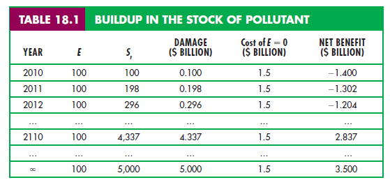
NUMERICAL EXAMPLE We can make this concept more concrete with a simple example. Suppose that, absent government intervention, 100 units of a pollutant will be emitted into the atmosphere every year for the next 100 years; the rate at which the stock dissipates, S, is 2 percent per year, and the stock of pollutant is initially zero. Table 18.1 shows how the stock builds up over time. Note that after 100 years, the stock will reach a level of 4,337 units. (If this level of emissions continued forever, the stock will eventually approach E/S = 100/.02 = 5,000 units.)
Suppose that the stock of pollutant creates economic damage (in terms of health costs, reduced productivity, etc.) equal to $1 million per unit. Thus, if the total stock of pollutant were, say, 1000 units, the resulting economic damage for that year would be $1 billion. And suppose that the annual cost of reducing emissions is $15 million per unit of reduction. Thus, to reduce emissions from 100 units per year to zero would cost 100 X $15 million = $1.5 billion per year. Would it make sense, in this case, to reduce emissions to zero starting immediately?
To answer this question, we must compare the present value of the annual cost of $1.5 billion with the present value of the annual benefit resulting from a reduced stock of pollutant. Of course, if emissions were reduced to zero starting immediately, the stock of pollutant would likewise be equal to zero over the entire 100 years. Thus, the benefit of the policy would be the savings of social cost associated with a growing stock of pollutant. Table 18.1 shows the annual cost of reducing emissions from 100 units to zero, the annual benefit from averting damage, and the annual net benefit (the annual benefit net of the cost of eliminating emissions). As you would expect, the annual net benefit is negative in the early years because the stock of pollutant is low; the net benefit becomes positive only later, after the stock of pollutant has grown.
To determine whether a policy of zero emissions makes sense, we must calculate the NPV of the policy, which in this case is the present discounted value of the annual net benefits shown in Table 18.1. Denoting the discount rate by R, the NPV is:
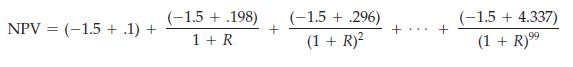
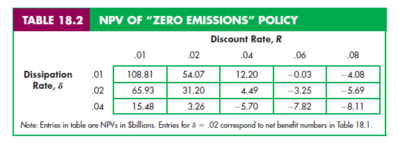
Is this NPV positive or negative? The answer depends on the discount rate, R. Table 18.2 shows the NPV as a function of the discount rate. (The middle row of Table 18.2, in which the dissipation rate 8 is 2 percent, corresponds to Table 18.1. Table 18.2 also shows NPVs for dissipation rates of 1 percent and 4 percent.) For discount rates of 4 percent or less, the NPV is clearly positive, but if the discount rate is large, the NPV will be negative.
Table 18.2 also shows how the NPV of a “zero emissions” policy depends on the dissipation rate, 8. If 8 is lower, the accumulated stock of pollutant will reach higher levels and cause more economic damage, so the future benefits of reducing emissions will be greater. Note from Table 18.2 that for any given discount rate, the NPV of eliminating emissions is much larger if S = .01 and much smaller if S = .04. As we will see, one of the reasons why there is so much concern over global warming is the fact that the stock of GHGs dissipates very slowly; S is only about .005.
Formulating environmental policy in the presence of stock externalities therefore introduces an additional complicating factor: What discount rate should be used? Because the costs and benefits of a policy apply to society as a whole, the discount rate should likewise reflect the opportunity cost to society of receiving an economic benefit in the future rather than today. This opportunity cost, which should be used to calculate NPVs for government projects, is called the social rate of discount. But as we will see in Example 18.5, there is little agreement among economists as to the appropriate number to use for the social rate of discount.
In principle, the social rate of discount depends on three factors: (1) the expected rate of real economic growth; (2) the extent of risk aversion for society as a whole; and (3) the “rate of pure time preference” for society as a whole. With rapid economic growth, future generations will have higher incomes than current generations, and if their marginal utility of income is decreasing (i.e., they are risk-averse), their utility from an extra dollar of income will be lower than the utility to someone living today; that’s why future benefits provide less utility and should thus be discounted. In addition, even if we expected no economic growth, people may simply prefer to receive a benefit today than in the future (the rate of pure time preference). Depending on one’s beliefs about future real economic growth, the extent of risk aversion for society as a whole, and the rate of pure time preference, one could conclude that the social rate of discount should be as high as 6 percent—or as low as 1 percent. And herein lies the difficulty. With a discount rate of 6 percent, it is hard to justify almost any government policy that imposes costs today but yields benefits only 50 or 100 years in the future (e.g., a policy to deal with global warming). Not so, however, if the discount rate is only 1 or 2 percent. Thus for problems involving long time horizons, the policy debate often boils down to a debate over the correct discount rate.
Source: Pindyck Robert, Rubinfeld Daniel (2012), Microeconomics, Pearson, 8th edition.
fabulous content