Cox Proportional Hazard Models by using Stata

Regression methods allow us to take survival analysis further and examine the effects of multiple continuous or categorical predictors. One widely-used method known as Cox regression employs a proportional hazard model. The hazard rate for failure at time t is defined as the rate of failures at time t among those who have survived to time t:

We model this hazard rate as a function of the baseline hazard (h ₀ ) at time t, and the effects of one or more x variables,

or, equivalently,

“Baseline hazard” means the hazard for an observation with all x variables equal to 0. Cox regression estimates this hazard nonparametrically and obtains maximum-likelihood estimates of the P parameters in [10.3]. Stata’s stcox procedure ordinarily reports hazard ratios, which are estimates of exp(P). These indicate proportional changes relative to the baseline hazard rate.

Does age affect the onset of AIDS symptoms? Dataset aids.dta contains information that addresses this question. Note that with stcox , unlike most other Stata model-fitting commands, we list only the independent variable(s). The survival-analysis dependent variables, time variables and censoring variables are understood automatically with stset data.

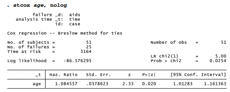
We might interpret the estimated hazard ratio, 1.084557, with reference to two HIV-positive individuals whose ages are a and a + 1. The older person is 8.5% more likely to develop AIDS symptoms over a short period of time (that is, the ratio of their respective hazards is 1.084557). This ratio differs significantly (p = .02) from 1. If we wanted to state our findings for a five-year difference in age, we could raise the hazard ratio to the fifth power:

Thus, the hazard of AIDS onset is about 50% higher when the second person is five years older than the first. Alternatively, we could learn the same thing (and obtain the new confidence interval) by repeating the regression after creating a new version of age measured in five-year units. The nolog noshow options below suppress display of the iteration log and the st-dataset description.

Like ordinary regression, Cox models can have more than one independent variable. Dataset heart.dta contains survival-time data from Selvin (1995) on 35 patients with very high cholesterol levels. Variable time gives the number of days each patient was under observation. coronary indicates whether a coronary event occurred at the end of this time period (coronary = 1) or not (coronary = 0). The data also include cholesterol levels and other factors thought to affect heart disease. File heart.dta was previously set up for survival-time analysis by an stset time, failure(coronary) command, so we can go directly to st analysis.

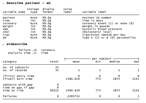
Cox regression finds that cholesterol level and cigarettes both significantly increase the hazard of a coronary event. Counterintuitively, weight appears to decrease the hazard. Systolic blood pressure and A/B personality do not have significant net effects.

After estimating the model, we can predict new variables holding the estimated baseline cumulative hazard and survivor functions. Since “baseline” refers to a situation with all x variables equal to zero, however, we first need to center some variables so that 0 values make sense. A patient who weighs 0 pounds, or has 0 blood pressure, does not provide a useful comparison. Guided by the minimum values actually in our data, we might shift weight so that 0 indicates 120 pounds, sbp so that 0 indicates 105, and chol so that 0 indicates 340: . summarize patient – ab

Zero values for all the x variables now make real-world sense. To create new variables holding the baseline survivor and cumulative hazard function estimates, we repeat the regression and follow this by two predict commands:

Note that centering three x variables had no effect on the hazard ratios, standard errors and so forth. The predict commands created two new variables, arbitrarily named hazard and survivor. To graph the baseline survivor function, we plot survivor against time and connect data points in a stairstep fashion, as seen in Figure 10.3.

The baseline survivor function — which depicts survival probabilities for patients having “0” weight (120 pounds), “0” blood pressure (105), “0” cholesterol (340), 0 cigarettes per day, and a type B personality — declines with time. Although this decline looks precipitous at the right, notice that the probability really only falls from 1 to about .96. Given less favorable values of the predictor variables, the survival probabilities would fall much faster.

The same baseline survivor-function graph could have been obtained another way, without stcox. The alternative, shown in Figure 10.4, employs an sts graph command with adjustfor( ) option listing the predictor variables.

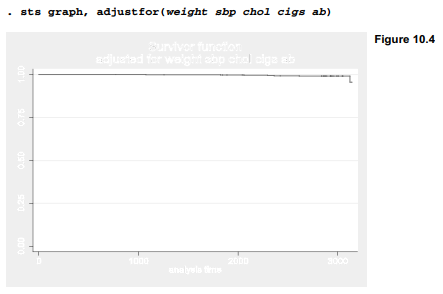
Figure 10.4, unlike Figure 10.3, follows the usual survivor-function convention of scaling the vertical axis from 0 to 1. Apart from this difference in scaling, Figures 10.3 and 10.4 depict the same curve.

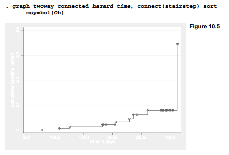
Figure 10.5 graphs the estimated baseline cumulative hazard against time, using the variable (hazard) generated by our stcox command. This graph shows the baseline cumulative hazard increasing in 8 steps (because 8 patients “failed” or had coronary events), from near 0 to .033.

Source: Hamilton Lawrence C. (2012), Statistics with STATA: Version 12, Cengage Learning; 8th edition.