Poisson Regression by using Stata

If events occur independently and with constant rate, then counts of events over a given period of time follow a Poisson distribution. Let r j represent the incidence rate:

The denominator in [10.4] is termed the “exposure” and is often measured in units such as person-years. We model the logarithm of incidence rate as a linear function of one or more predictors:

Equivalently, the model describes logs of expected event counts:

Assuming that a Poisson process underlies the events of interest, Poisson regression finds maximum-likelihood estimates of the P parameters.

Data on radiation exposure and cancer deaths among workers at Oak Ridge National Laboratory provide an example. The 56 observations in dataset oakridge.dta represent 56 age/radiation- exposure categories (7 categories of age x 8 categories of radiation exposure). For each combination, we know the number of deaths and the number of person-years of exposure.

. use C:\data\oakridge.dta, clear

Does the death rate increase with exposure to radiation? Poisson regression finds a statistically significant effect:

For the regression above, we specified the event count (deaths) as the dependent variable and radiation (rad) as the independent variable. The Poisson exposure variable ispyears, or person- years in each category of rad. The irr option calls for incidence rate ratios rather than regression coefficients in the results table — that is, we get estimates of exp(P) instead of P, the default. According to this incidence rate ratio, the death rate becomes 1.236 times higher (increases by 23.6%) with each increase in radiation category. Although that ratio is statistically significant, the fit is not impressive. The pseudo R² (equation [9.4]) is only .042.

To perform a goodness-of-fit test, comparing the Poisson model’s predictions with the observed counts, use the postestimation command estat gof :

These goodness-of-fit test results indicate that our model’s predictions are significantly different from the actual counts — another sign that the model fits poorly.

We obtain better results when we include age as a second predictor. Pseudo R² then rises to .5966, and the goodness-of-fit test no longer leads to rejecting our model.

For simplicity, to this point we have treated rad and age as if both were continuous variables, and we expect their effects on the log death rate to be linear. In fact, however, both independent variables are measured as ordered categories. rad = 1, for example, means 0 radiation exposure; rad = 2 means 0 to 19 millisieverts; rad = 3 means 20 to 39 millisieverts; and so forth. An alternative way to include radiation exposure categories in the regression, while watching for nonlinear effects, is as a set of indicator variables using Stata’s factor-variable notation. The i.rad term in the following model specifies that a {0, 1} indicator for each category of rad be included along with age as predictors. rad = 1 is automatically omitted as the base category.

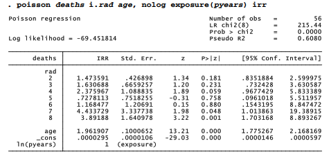
The additional complexity of this indicator-variable model brings little improvement in fit. It does, however, add to our interpretation. The overall effect of radiation on death rate appears to come primarily from the two highest radiation levels (rad = 7 and rad = 8, corresponding to 100 to 119 and 120 or more milliseiverts). At these levels, the incidence rates are about four times higher.

Radiation levels 7 and 8 seem to have similar effects, so we might simplify the model by combining them. First, we test whether their coefficients are significantly different. They are not: . test 7.rad = 8.rad

Next, generate a new dummy variable rad78, which equals 1 if rad equals 7 or 8. Substitute this new variable for the separate rad = 7 and rad = 8 indicators. The commands illustrate how to do so in factor-variable notation.

. generate rad78 = (7.rad | 8.rad)

. poisson deaths i(1/6).rad rad78 age, irr ex(pyears) nolog

We could proceed to simplify the model further in this fashion. At each step, test helps to evaluate whether combining two dummy variables is justifiable.

Source: Hamilton Lawrence C. (2012), Statistics with STATA: Version 12, Cengage Learning; 8th edition.