Data that were previously saved in Stata format can be retrieved into memory either by typing a command of the form use filename, or by menu selections. This section describes basic tricks for creating Stata-format datasets in the first place. We could start simply by typing data into the Data Editor by hand. A by-hand approach is practical with small datasets, or may be unavoidable when the original information is printed material such as a table in a book. If the original information is in electronic format such as a text file or spreadsheet, however, more direct approaches are possible.
Table 2.1 lists some information about Canadian provinces and territories that can be used to illustrate the by-hand approach. These data are from the Federal, Provincial and Territorial Advisory Committee on Population Health, 1996. Canada’s newest territory, Nunavut, is not listed here because it was part of the Northwest Territories until 1999.
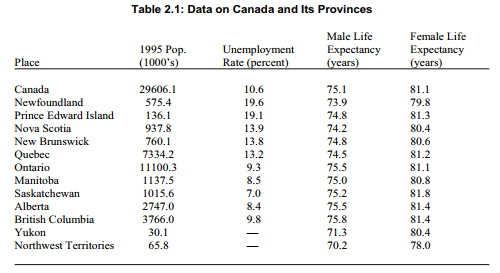
The simplest way to create a dataset from printed information like Table 2.1 is through the Data Editor, invoked by clicking , selecting Window > Data Editor from the menu bar, or by typing the command edit. Then begin typing values for each variable, in columns initially labeled varl, var2 etc. Thus, varl contains place names, var2 populations, and so forth.
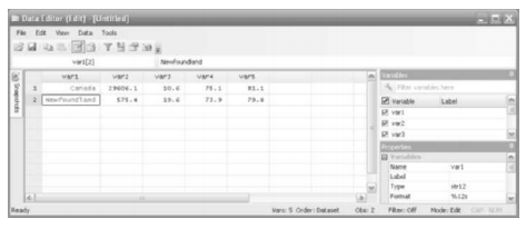
We can assign more descriptive variable names by double-clicking on the column headings (such as varl) and then typing a new name in the resulting dialog box; eight characters or fewer works best, although names with up to 32 characters are allowed. We can also create variable labels that contain a brief description. For example, var2 (population) might be renamed pop, and given the variable label “Population in 1000s, 1995”.
Renaming and labeling variables can also be done outside of the Data Editor through the rename and label variable commands:
. rename var2 pop
. label variable pop “Population in 1000s, 1995”
Cells left empty, such as unemployment rates for the Yukon and Northwest Territories, will automatically be assigned Stata’s default missing value code, a period. At any time, we can close the Data Editor and then save the dataset to disk. Clicking or Data > Data Editor, or typing the command edit, brings the Editor back.
If the first value entered for a variable is a number, as with population, unemployment and life expectancy, then Stata assumes that this column is a numeric variable and it will thereafter permit only numbers as values. Numeric values can also begin with a plus or minus sign, include decimal points, or be expressed in scientific notation. For example, we could represent Canada’s population as 2.96061e+7, which means 2.96061 x 10⁷ or about 29.6 million people. Numbers should not include any commas, such as 29,606,100 (or using commas as a decimal separator). If we did happen to put commas within the first value typed in a column, Stata would interpret this as a string variable (next paragraph) rather than as a number.
If the first value entered for a variable includes non-numeric characters, as did place names above (or “1,000” with the comma), then Stata thereafter considers this column to be a string or text variable. String variable values can be almost any combination of letters, numbers, symbols or spaces up to 244 characters long. They can store names, quotations or other descriptive information. String variable values could be tabulated and counted, but not analyzed using means, correlations or most other statistics. In the Data Editor or Data Browser, string variable values appear in red, distinguishing them from numeric (black) or labeled numeric (blue) variables.
After typing in the information from Table 2.1 in this fashion, we close the Data Editor and save our data, perhaps with the name Canadal.dta:
. save Canadal
Stata automatically adds the extension .dta to any dataset name, unless we tell it to do otherwise. If we already had saved and named an earlier version of this file, it is possible to write over that with the newest version by typing
. save, replace
At this point, our new dataset looks like this:
. describe
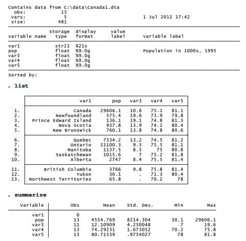
Examining such output gives us a chance to look for errors that should be corrected. The summarize table, for instance, provides several numbers useful in proofreading, including the count of nonmissing numerical observations (always 0 for string variables) and the minimum and maximum for each variable. Substantive interpretation of the summary statistics would be premature at this point, because our dataset contains one observation (Canada) that represents a combination of the other 12 provinces and territories.
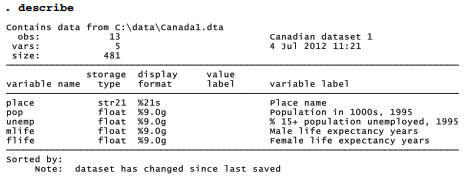
The next step is to make our dataset more self-documenting. The variables could be given more descriptive names, such as the following:
. rename var1 place
. rename var3 unemp
. rename var4 mlife
. rename var5 flife
Alternatively, the four rename operations could be accomplished in one step:
. rename (varl var2 var3 var4) (place unemp mlife flife)
Stata also permits us to add several kinds of labels to the data. label data describes the dataset as a whole, whereas label variable describes an individual variable. For example,
. label data “Canadian dataset 1”
. label variable place “Place name”
. label variable unemp “% 15+ population unemployed, 1995”
. label variable mlife “Male life expectancy years”
. label variable flife “Female life expectancy years”
By labeling data and variables, we obtain a dataset that is more self-explanatory:
Once labeling is completed, we should save the data to disk by using File > Save or typing
. save, replace
We could later retrieve these data any time through ![]() , File > Open, or by typing
, File > Open, or by typing
. use C:\data\Canada1
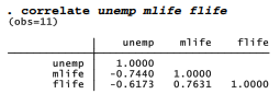
Now we can proceed with analysis. We might notice, for instance, that male and female life expectancies correlate positively with each other and also negatively with the unemployment rate. The life expectancy-unemployment rate correlation is stronger for males.
The order of observations within a dataset can be changed by the sort command. For example, to rearrange observations from smallest to largest in population, type
. sort pop
String variables are sorted alphabetically instead of numerically. Typing sort place will rearrange observations putting Alberta first, British Columbia second, and so on.
The order command controls the order of variables within a dataset. For example, we could make unemployment the second variable, and population last:
. order place unemp mlife flife pop
The Data Editor also offers a Tools menu with choices that can perform these operations.
We can restrict the Data Editor beforehand to work only with certain variables, in a specified order, or with a specified range of values. For example,
. edit place mlife flife or . edit place unemp if pop > 100
The last example employs an if qualifier, an important tool described in later sections.
Source: Hamilton Lawrence C. (2012), Statistics with STATA: Version 12, Cengage Learning; 8th edition.
3 Oct 2022
3 Oct 2022
30 Sep 2022
3 Oct 2022
3 Oct 2022
29 Sep 2022