Monte Carlo Simulation by using Stata

Monte Carlo simulations generate and analyze many samples of artificial data, allowing researchers to investigate the long-run behavior of their statistical techniques. The simulate command makes designing a simulation straightforward so that it only requires a small amount of additional programming. This section gives two examples.

To begin a simulation, we need to define a program that generates one sample of random data, analyzes it, and stores the results of interest in memory. The following file defines an r-class program (one capable of storing r( ) results) named meanmedian. This program randomly generates 100 values of variable x from a standard normal distribution. It next generates 100 values of variable w from a contaminated normal distribution: N(0,1) with probability .95, and N(0,10) with probability .05. Contaminated normal distributions have often been used in robustness studies to simulate variables that contain occasional wild errors. For both variables, meanmedian obtains means and medians.

• Creates a sample containing n=100 observations of variables x and w.
• x~N(0,1) x is standard normal
• w~N(0,1) with p=.95, w~N(0,10) with p=.05 w is contaminated normal
• Calculates the mean and median of x and w.
• Stored results: r(xmean) r(xmedian) r(wmean) r(wmedian)

program meanmedian, rclass

version 12.1

drop _all

set obs 100

generate x = rnormal()

summarize x, detail

return scalar xmean = r(mean)

return scalar xmedian = r(p50)

generate w = rnormal()

replace w = 10*w if runiform() < .05

summarize w, detail

return scalar wmean = r(mean)

return scalar wmedian = r(p50)

end

Because we defined meanmedian as an r-class command, like summarize, it can store its results in r( ) scalars. meanmedian creates four such scalars: r(xmean) and r(xmedian) for the mean and median of x; r(wmean) and r(wmedian) for the mean and median of w.

Once meanmedian has been defined, whether through a do-file, ado-file, or typing commands interactively, we can call this program with a simulate command. To create a new dataset containing means and medians of x and w from 5,000 random samples, type

. simulate xmean = r(xmean) xmedian = r(xmedian) wmean = r(wmean)

wmedian = r(wmedian), reps(5000): meanmedian

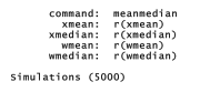
This command creates new variables xmean, xmedian, wmean and wmedian, based on the r( ) results from each iteration of meanmedian.

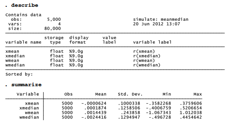
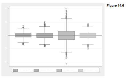
The means of these means and medians, across 5,000 samples, are all close to 0 — consistent with our expectation that the sample mean and median should both provide unbiased estimates of the true population means (0) for x and w. Also as theory predicts, the mean exhibits less sample-to-sample variation than the median when applied to a normally distributed variable (x). The standard deviation of xmedian is .126, noticeably larger than the standard deviation of xmean (.100). When applied to the non-normal, outlier-prone variable w, on the other hand, the opposite holds true: the standard deviation of wmedian is much lower than the standard deviation of wmean (.129 versus .244). This Monte Carlo experiment demonstrates that the median remains a relatively stable measure of center despite wild outliers in the contaminated distribution, whereas the mean breaks down and varies much more from sample to sample. Figure 14.6 draws the comparison graphically as box plots (and, incidentally, demonstrates how to control the shapes of box plot outlier-marker symbols). To make room for four variables within the one-row legend, symbols are drawn with only half their usual width (symxsize(*.5)).

. graph box xmean xmedian wmean wmedian, yline(0)

legend(row(1) symxsize(*.5))

marker(1, msymbol(+)) marker(2, msymbol(Th))

marker(3, msymbol(Oh)) marker(4, msymbol(Sh))

Our next example extends the inquiry to robust methods, bringing together several themes from this book. Program regsim generates 100 observations of x (standard normal) and two y variables. y1 is a linear function of x plus standard normal errors. y2 is also a linear function of x, but adding contaminated normal errors. These variables help to explore how various regression methods behave in the presence of normal and nonnormal, heavy-tailed error distributions. Four methods are employed: ordinary least squares (regress), robust regression (rreg), quantile regression (qreg), and quantile regression with bootstrapped standard errors (bsqreg, with 500 repetitions). Robust and quantile regression (Chapter 8) in theory should prove more resistant to the effects of outliers. Through this Monte Carlo experiment, we test whether that is true. regsim applies each method to the regression of y1 on x and then to the regression ofy2 on x. For this exercise, the program is defined by an ado-file, regsim.ado, saved in the ado\personal directory.

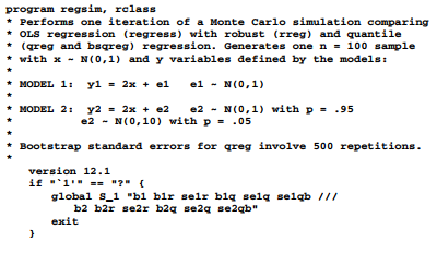
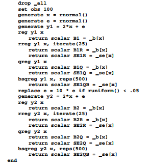
The r-class program stores coefficient or standard error estimates from eight regression analyses. These results are given names such as

r(B1) coefficient from OLS regression of y1 on x

r(B1R) coefficient from robust regression of y1 on x

r(SE1R) standard error of robust coefficient from model 1

and so forth. All the robust and quantile regressions involve multiple iterations: typically five to ten iterations for rreg, about five for qreg, and several thousand for bsqreg with its 500 bootstrap re-estimations of about five iterations each, per sample. Thus, a single execution of regsim demands more than 2,000 regressions. The following command calls for five repetitions, requiring more than 10,000 regressions.

. simulate b1 = r(B1) blr = r(B1R) selr = r(SE1R)

blq = r(B1Q) selq = r(SE1Q) selqb = r(SE1QB) b2 = r(B2)

b2r = r(B2R) se2r = r(SE2R) b2q = r(B2Q) se2q = r(SE2Q)

se2qb = r(SE2QB), reps(5): regsim

You might want to run a small simulation like this as a trial to get a sense of the time required on your computer. For research purposes, however, we would need a larger experiment. Dataset regsim.dta contains results from an experiment involving 500 repetitions of regsim — more than a million regressions. The regression coefficients and standard error estimates produced by this experiment are summarized below.

. describe

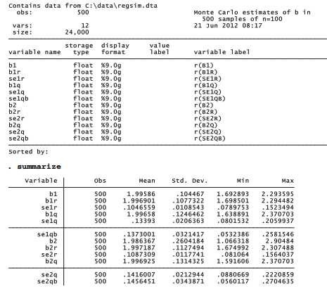
Figure 16.8 draws the distributions of coefficients as box plots. To make the legend readable we use the legend(symxsize(*.3) colgap(*.3)) options, which set the width of symbols and the gaps between columns within the legend at just 30% of their default size. help legend option and help relativesize supply further information about these options.

.graph box bl blr blq b2 b2r b2q,

ytitle(“Estimates of slope (b=2)”>

yline(2) legend(row(1) symxsize(*.3) colgap(*.3)

label(3 “quantile 1”) label(6 “quantile 2”))

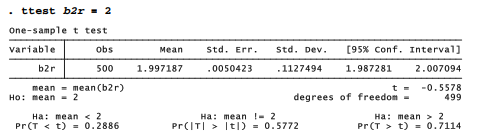
All three regression methods (OLS, robust and quantile) produced mean coefficient estimates for both models that are not significantly different from the true value, P = 2. This can be confirmed through t tests such as

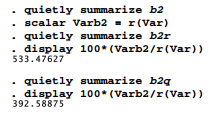
All the regression methods thus yield unbiased estimates of P, but they differ in their sample-to- sample variation or efficiency. Applied to the normal-errors model 1, OLS proves the most efficient, as the Gauss-Markov theorem predicts. The observed standard deviation of OLS coefficients is .1045, compared with .1077 for robust regression and .1246 for quantile regression. Relative efficiency, expressing an OLS coefficient’s observed variance as a percentage of another estimator’s variance, provides a standard way to compare such statistics:

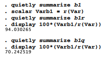
The calculations above use the r(Var) variance result from summarize. We first obtain the variance of the OLS estimates b1, and make this value scalar Varbl. Next the variances of the robust estimates blr, and the quantile estimates blq, are obtained and each is compared with Varbl. This reveals that robust regression was about 94% as efficient as OLS when applied to the normal-errors model — close to the large-sample efficiency of 95% that this robust method theoretically should have (Hamilton 1992a). Quantile regression, in contrast, achieves a relative efficiency of only 70% with the normal-errors model.

Similar calculations for the contaminated-errors model tell a different story. OLS was the best (most efficient) estimator with normal errors, but with contaminated errors it becomes the worst:

Outliers in the contaminated-errors model cause OLS coefficient estimates to vary wildly from sample to sample, as can be seen in the fourth box plot of Figure 14.7. The variance of these OLS coefficients is more than five times greater than the variance of the corresponding robust coefficients, and almost four times greater than that of quantile coefficients. Put another way, both robust and quantile regression prove to be much more stable than OLS in the presence of outliers, yielding correspondingly lower standard errors and narrower confidence intervals. Robust regression outperforms quantile regression with both the normal-errors and the contaminated-errors models.

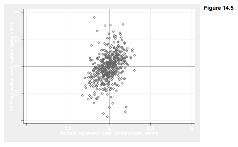
Figure 14.8 illustrates the comparison between OLS and robust regression with a scatterplot showing 500 pairs of regression coefficients. The OLS coefficients (vertical axis) vary much more widely around the true value, 2.0, than rreg coefficients (horizontal axis) do.

. graph twoway scatter b2 b2r, msymbol(dh) ylabel(1(.5)3, grid)

yline(2) xlabel(1(.5)3, grid gmin gmax) xline(2)

ytitle(“OLS regression coef, contaminated errors”)

xtitle(“Robust regression coef, contaminated errors”)

The Monte Carlo experiment also provides information about the estimated standard errors under each method and model. Mean estimated standard errors differ from the observed standard deviations of coefficients. Discrepancies for the robust standard errors are relatively small — less than 4%. For the theoretically-derived quantile standard errors the discrepancies are larger, around 7%. The least satisfactory estimates appear to be the bootstrapped quantile standard errors obtained by bsqreg. Means of the bootstrap standard errors exceed the observed standard deviation of blq and b2q by 10 or 11%. Bootstrapping apparently over-estimates the sample-to- sample variation.

Monte Carlo simulation has become a key method in modern statistical research, and it plays a growing role in statistical teaching as well. These examples demonstrate some easy ways to get started.

Source: Hamilton Lawrence C. (2012), Statistics with STATA: Version 12, Cengage Learning; 8th edition.