Analysis of variance (ANOVA) provides another way, more general than t tests, to test for differences among means. The simplest case, one-way ANOVA, tests whether the means of y differ across categories of x. One-way ANOVA can be performed by a oneway command with the general form oneway measurement categorical. For example,

The tabulate option produces a table of means and standard deviations in addition to the analysis of variance table itself. One-way ANOVA with a dichotomous x variable is equivalent to a two-sample t test, and its F statistic equals the corresponding t statistic squared. oneway offers more options and processes faster, but it lacks an unequal option for relaxing the equal- variances assumption.
oneway does, however, formally test the equal-variances assumption using Bartlett’s /2. A low Bartlett’s probability implies that an equal-variance assumption is implausible, in which case we should not trust the ANOVA F test results. In the oneway drink belong example above, Bartlett’s p = .028 casts doubt on the ANOVA’s validity.
One-way ANOVA’s real value lies not in two-sample comparisons, but in comparisons of three or more means. For example, we could test whether mean drinking behavior varies by year in college. The term “freshman” refers to first-year students, not necessarily male.
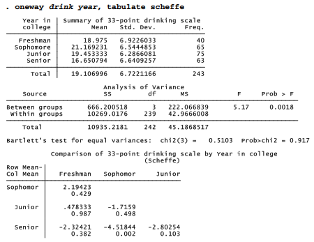
We can reject the hypothesis of equal means (p = .0018), but not the hypothesis of equal variances (p = .917). The latter is good news regarding the ANOVA’s validity.
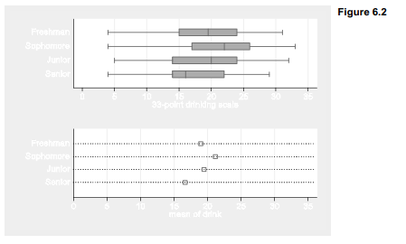
The horizontal box plots (graph hbox) in Figure 6.2 support this conclusion, showing similar variation within each category. For this image the box plots are combined with a dot chart (graph dot (mean)) depicting means within each category. The combined image shows that differences among medians (top) and differences among means (bottom) follow similar patterns. Dot charts serve much the same purpose as bar charts: visually comparing statistical summaries of one or more measurement variables. The organization and options for dot charts and bar charts are broadly similar, including the choices of statistical summaries. Type help graph dot for details.
. graph hbox drink, over(year) ylabel(0(5)35) saving(fig06_02a)
. graph dot (mean) drink, over(year) ylabel(0(5)35, grid) marker(1, msymbol(Sh)) saving(fig06_02b)
. graph combine fig06_02a.gph fig06_02b.gph, row(2) iscale(1.05)
The scheffe option (Scheffe multiple-comparison test) with our oneway command produced a table showing the differences between each pair of means. The freshman mean equals 18.975 and the sophomore mean equals 21.16923, so the sophomore-freshman difference is 21.16923 – 18.975 = 2.19423, not statistically distinguishable from zero (p = .429). Of the six contrasts in this table, only the senior-sophomore difference, 16.6508 – 21.1692 = -4.5184, is significant (p = .002). Thus, our overall conclusion that these four groups’ means are not the same arises mainly from the contrast between seniors (the lightest drinkers) and sophomores (the heaviest).
oneway offers three multiple-comparison options: scheffe, bonferroni and sidak (see Base Reference Manual for definitions). The Scheffe test remains valid under a wider variety of conditions, although it is sometimes less sensitive.
The Kruskal-Wallis test (kwallis), a ^-sample generalization of the two-sample rank-sum test, provides a nonparametric alternative to one-way ANOVA. It tests the null hypothesis of equal population medians.
. kwallis drink, by(year)

These kwallis results (p = .0023) agree with our oneway findings of significant differences in drink by year in college. Kruskal-Wallis is generally safer than ANOVA if we have reason to doubt ANOVA’s equal-variances or normality assumptions, or if we suspect problems caused by outliers. kwallis, like ranksum, makes the weaker assumption of similar-shaped rank distributions within each group. In principle, ranksum and kwallis should produce similar results when applied to two-sample comparisons, but in practice this is true only if the data contain no ties. ranksum incorporates an exact method for dealing with ties, which makes it preferable for two-sample problems.
Source: Hamilton Lawrence C. (2012), Statistics with STATA: Version 12, Cengage Learning; 8th edition.
23 Sep 2022
3 Oct 2022
26 Sep 2022
24 Sep 2022
28 Sep 2022
29 Sep 2022