predict can also calculate many other case statistics appropriate for the recently-fitted model. After regress (or anova), predict options include the following. Substitute any new variable name for new in these examples.
. predict new Predicted values of y. predict new, xb means the same thing (referring to Xb, the vector of predicted y values).
. predict new, resid Residuals.
. predict new, rstandard Standardized residuals.
. predict new, rstudent Studentized (jackknifed) residuals, measuring the ith observation’s influence on the y-intercept.
. predict new, rstudent Standard errors of predicted mean y.
. predict new, stdf Standard errors of predicted individual y, sometimes called the standard errors of forecast or the standard errors of prediction.
. predict new, hat Diagonal elements of hat matrix (leverage also works).
. predict new, cooksd Cook’s D influence, measuring the zth observation’s influence on all coefficients in the model (or, equivalently, on all n predicted y values).
Further options obtain predicted probabilities and expected values; type help regress for a list.
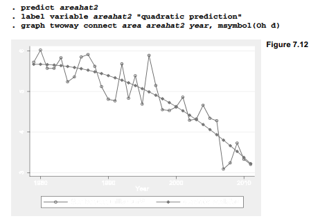
For illustration, we return to the trend in Arctic sea ice (Arctic9.dta). Residual analysis in the previous section suggests that a linear model, Figure 7.9, is not appropriate for these data. One simple alternative termed quadratic regression involves regressing the dependent variable on both year and year squared. We could start by generating a new variable equal to year squared:
. generate year2 = year^2
. regress area year year2

This quadratic regression displays an overall improvement in fit: R2a = .8066, compared with .7549 for the linear regression. Moreover, the improvement is statistically significant, as evidenced by the significant coefficient on year2 (p = .005). A scatterplot (Figure 7.12) visualizes this improvement: the quadratic model does not systematically over- then under- then over-predict the actual ice area, as happened with our previous linear model.
Two alternative ways to conduct the same quadratic regression, without first generating a new variable for year squared, would be to use Stata’s interaction (#) notation. All three of the following commands estimate the same model. Either of the # versions would be needed for a subsequent margins command to work properly.
. regress area year year2
. regress area year c.year#c.year
. regress area c.year##c.year
Although improvement visible in Figure 7.12 is encouraging, quadratic regression can introduce or worsen some statistical problems. One such problem is leverage, meaning the potential influence of observations with unusual x values, or unusual combinations of x values. Leverage statistics, also called hat matrix diagonals, can be obtained by predict. In this example we unimaginatively name the leverage measure leverage.
. predict leverage, hat
Figure 7.13 draws the quadratic regression curve again, this time making the area of connect marker symbols proportional to leverage by specifying analytical weights, [aw=leverage]. This graph also overlays a median spline plot (mspline) which draws a smooth curve connecting the predicted values areahat2. Median spline plots often serve better than line or connected-line plots to graph a curvilinear relationship. For this purpose it helps to specify a large number of bands(); type help twoway mspline for more about this twoway plot type.

The marker symbols in Figure 7.13 are largest for the first and last years, because these have the most leverage. Quadratic regression tends to exaggerate the importance of extreme x values (which, through squaring, become even more extreme) so the model tracks those values closely. Note how well the curve fits the first and last years.
Leverage reflects the potential for influence. Other statistics measure influence directly. One type of influence statistic, DFBETAS, indicates by how many standard errors the coefficient on x1 would change if observation i were dropped from the regression. These can be obtained for
a single predictor through a predict new, dfbeta(xvarname) command. DFBETAS for all of the predictors in a model are obtained more easily by the dfbeta command, which creates a new variable for each predictor. In our example there are two predictors, year and year2. Consequently the dfbeta command defines two new influence statistics, one for each predictor.

Box plots in Figure 7.14 show the distributions of both DFBETAS variables, with outliers labeled by year.

The _dfbeta_1 values measure the influence of each observation on the coefficient for year. 1996 (visible as a particularly high value in Figure 7.13) exerts the most influence on the year coefficient. The dfbetal = .55 tells us that the coefficient on year in the full-sample regression is about .55 standard errors higher than it would be, if we re-estimated the model with 1996 set aside. Similarly, the negative value for 1980, _dfbeta_1 = -.336, indicates that the full-sample coefficient on year is about .336 standard errors lower than it would be, if we re-estimated the model with 1980 set aside. And while 1996 makes the coefficient on year higher than it would
otherwise be, it makes the coefficient onyear2 lower by a similar amount. The reverse applies to 1980. In the original data (Figure 7.13) 1980 is not much of an outlier, but it has relatively high leverage which makes it more influential than other equally outlying but lower-leverage years.
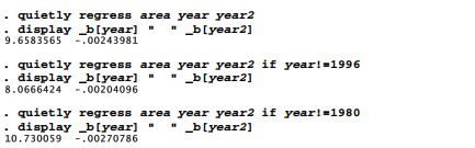
If we were unsure about how to read DFBETAS, we could confirm our interpretation by repeating the regression with influential observations set aside. To save space, quietly here suppresses the regression output, and we ask only to display the coefficients on year and year2, separated by two blank spaces for readability. The first regression employs the full sample. The second sets aside 1996, which makes the coefficient on year lower (from 9.658 to 8.067) and the coefficient on year2 higher (from -.0024 to -.0020). Setting aside 1980 in the third regression has an opposite effect: the coefficient on year becomes higher (9.658 to 10.730) and the coefficient on year2 becomes lower (-.0024 to -.0027).
If we use # to enter the squared term instead, the last commands would be as follows.
![]()
Leverage, DFBETAS or any other case statistic could be used directly to exclude observations from an analysis. For example, the first two commands below calculate Cook’s D, a statistic that measures influence of each observation on the model as a whole, instead of on individual coefficients as DFBETAS do. The third command repeats the initial regression using only those observations with Cook’s D values below .10.
. regress area year year2
. predict D, cooksd
. regress area year year2 if D <.10
Using any fixed definition of what constitutes an outlier, we are liable to see more of them in larger samples. For this reason, sample-size-adjusted cutoffs are sometimes recommended for identifying unusual observations. After fitting a regression model with K coefficients (including the constant) based on n observations, we might look more closely at those observations for which any of the following are true:

![]()
The reasoning behind these cutoffs, and the diagnostic statistics more generally, can be found in Cook and Weisberg (1982, 1994), Belsley, Kuh and Welsch (1980) or Fox (1991).
Source: Hamilton Lawrence C. (2012), Statistics with STATA: Version 12, Cengage Learning; 8th edition.
29 Sep 2022
30 Sep 2022
26 Sep 2022
26 Sep 2022
26 Sep 2022
26 Sep 2022