Opponents of technical analysis claim that looking at past technical data, such as price and volume, to help predict the future is outlandish. In the popular book A Random Walk Down Wall Street, Burton Malkiel refers to technical analysis as “sharing a pedestal with alchemy.” Some of these opponents believe that no underlying patterns exist in stock prices. These individuals believe that prices move in a random fashion and have no “memory.” This assumption would imply that technical analysis, which depends on prices predicting prices, has no foundation because all price motion is random.
A random walk occurs when future steps cannot be predicted by observing past steps. Each step is independent of all others. For example, flipping a coin produces a random walk. Suppose you flip a coin once and it lands on heads; observing that the coin landed on heads does not help you predict what the outcome will be the next time the coin is flipped. Each flip of the coin is an independent event, and the outcome of one flip of the coin has no impact on the outcome of any other flip. If the stock market follows a random walk, future stock prices cannot be predicted by observing past stock price movements.
The concept that stock price returns followed a random walk was first suggested by Louis Bachelier (see Box 4.1), a French mathematician, in his PhD thesis, “The Theory of Speculation” (1900, 1906, and 1913). He commented that “the mathematical expectation of the speculator is zero.” Although Bachelier described the concept, Karl Pearson, a Fellow of the Royal Society, introduced the term random walk in 1905 in Nature.
In the 1937 Econometrica article, “Some A Posteriori Probabilities in Stock Market Action,” Alfred Cowles and Herbert E. Jones (1937) also hypothesized that the stock market prices exhibited randomness. It was the 1964 book The Random Character of Stock Market Prices, edited by Paul Cootner, that popularized the random walk theory and its application in the stock market. The following year, Eugene Fama’s seminal article (1965) “The Behavior of Stock Market Prices” was published in the Journal of Business, giving additional credence to the random walk theory.
Box 4.1 Louis Bachelier
Louis Bachelier (1870-1946) was the first person to anticipate Brownian motion, random walk of financial prices, option pricing, and martingales long before Einstein, Wiener, and Black and Scholes. Receiving high marks from his advisor, the famous mathematician Henri Poincare, Bachelier became a lecturer at the Sorbonne and at several other universities. In 1926, he was turned down for a professorship at Dijon because of a critical letter from another famous mathematician, Paul Levy, who was unfamiliar with his earlier work. Later, in 1931, Levy learned of his work and sent an apology. Bachelier ended up as a professor in Besangon. Einstein had never heard of his work. Finally, in the 1960s, when Professor Paul Samuelson distributed Bachelier’s work among leading economists, his financial theories were “rediscovered.”
1. Fat Tails
A normal distribution curve looks like the bell-shaped chart in Figure 4.1. This normal, or Gaussian, distribution is often used in the natural and social sciences to represent real-valued random variables whose distributions are not known. (See Appendix A, “Basic Statistics,” for more information about the normal distribution.)
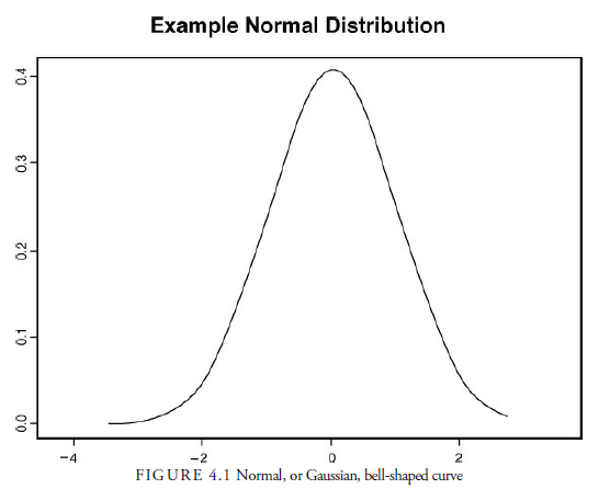
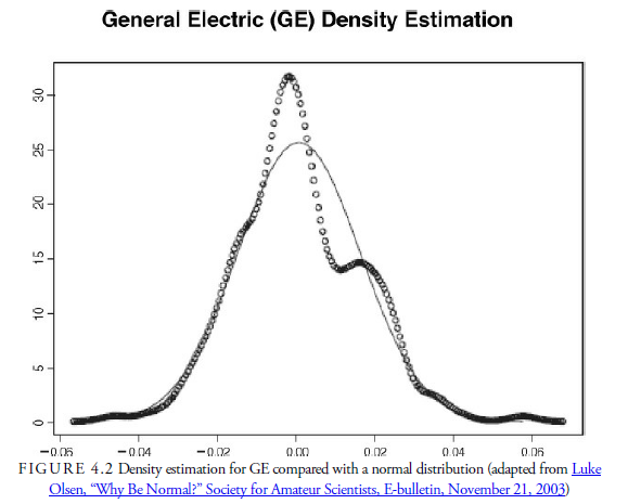
Figure 4.2 shows a chart of the actual distribution of stock returns for General Electric between January 1, 2003, and November 19, 2003. Compare Figure 4.1 with Figure 4.2. Notice how the chart of real historical returns (Figure 4.2) does not perfectly match the bell-shaped curve shown in Figure 4.1. In particular, compare the outer edges, or tails, of the two charts. The tails of the normal distribution, in Figure 4.1, get thinner and thinner, approaching zero. However, in the actual stock return data in Figure 4.2, we do not see this thinning of the tails; instead, we see that the tails have bumps or remain flat. Thus, “fat tails” are present in Figure 4.2 but not in Figure 4.1.
As early as 1915, Wesley C. Mitchell noticed that the distribution of price changes does not exactly follow the Gaussian distribution of Figure 4.1. Maurice Olivier, in his 1926 dissertation, and Frederick C. Mills, in The Behavior of Prices (1927), provided further evidence of a “leptokurtic distribution” of price changes. The leptokurtic distribution is more “pointed” than the normal, Gaussian, distribution. The leptokurtic distribution has a thinner peak and fatter tails than the normal, Gaussian, distribution. These fat tails indicate that stock prices are more likely to deviate extraordinarily from the mean more often than the normal, Gaussian, distribution of returns suggests.
Benoit Mandelbrot (1963) noted that stock market data collected since 1900 supported the observations of Mitchell and Mills. Concluding that market data differed enough from that assumed by a Gaussian distribution, Mandlebrot presented and tested a new model of price behavior, assuming a more general and stable Paretian distribution.
An example of one of these events is the large decline in stock prices that occurred on October 19, 1987. On this day, known as “Black Monday,” the U.S. stock market crashed, sending the Dow Jones Industrial Average down 22.6%. What are the chances of a one-day drop of this magnitude occurring randomly? In a 1996 article appearing in the Journal of Finance, Jens Carsten Jackwerth and Mark Rubenstein state that if the life of the universe had been repeated one billion times and the stock market were open every day, a crash of that magnitude would still have been “unlikely.” In his 2003 book Why Stock Markets Crash: Critical Events in Complex Financial Systems, Didier Sornette claims that, statistically, a crash as large as was seen on Black Monday would be expected to occur only once in 520 million years. Thus, the huge negative return seen in October 1987 is clearly an outlier.
Despite significant statistical evidence that stock returns do not follow a normal, Gaussian distribution, the properties of the normal distribution are often used to describe stock returns. Whether this is appropriate is subject to interpretation. The mathematics of the Gaussian distribution are easier to work with than that of other distributions; if the results of using a Gaussian distribution do not differ significantly from the results when more robust, exact assumptions are made, then using a simpler, Gaussian distribution may be appropriate. It is also important to note that the lack of stock returns following a normal distribution does not lead to the conclusion that stock returns are not random. Other distributions, including the leptokurtic, can result from random variables.
2. Large Unexpected Drawdowns
Black Monday represented an abnormally large one-day negative return in the stock market. Although this alone was a significant deviation from the mean stock return, even more significant is the fact that October 19 was preceded by three days of market losses. Market losses were 2%, 3%, and 6% on the three previous trading days. In other words, there were four consecutive days of trading losses, resulting in a 30% decline in the market. Periods of successive losses from a previous price peak are referred to as drawdo wns.
Sornette has studied these types of drawdowns in an attempt to understand why outliers occur and how they can be integrated into the RWH. He argues that although independence can accommodate one large deviation, the probability of two or more large deviations occurring back to back is out in the stratosphere.
For example, the probability of a one-day decline of 10% in the stock market is approximately 1 in 1,000. In other words, a 10% drop would occur statistically once every four years. Although a drop of this magnitude would be a large deviation from the average daily stock return, it would fall within the normal distribution. If stock returns are independent, the probability of two consecutive daily drops of 10% would be the product of the probability of the two independent events occurring, or 1/1000 multiplied by 1/1000. Likewise, the probability of three consecutive 10% drops, or a 30% drawdown, is 1/1000 x 1/1000 x 1/1000, or 1 in 1,000,000,000. This means, statistically, a 30% three-day drawdown could be expected to occur only once every four million years!
Historically, of course, these back-to-back events have occurred, especially in declines. Dismissing randomness under such events suggests that when sequential returns reach a critical mass, they begin to foretell future returns and are, thus, no longer random or independent. Sornette calls these periods bursts of dependence or pockets of predictability. If these successive declines occur more often than what is statistically predicted, some correlation must exist between the daily stock returns, indicating that stock returns do not follow a random walk.
As shown in Table 4.2, Sornette’s research indicates that large drawdowns in the DJIA have occurred more often than can be statistically expected. When considering the three largest twentieth-century stock market declines (1914, 1929, and 1987), Sornette calculates that statistically about 50 centuries should separate crashes of these magnitudes. He concludes that three declines of this magnitude occurring within three-quarters of a century of each other are an indication that the series of returns was not completely random.

What Sornette found was that under normal circumstances, returns follow a generally normal, Gaussian distribution. These normal conditions represent about 99% of market drawdowns. However, there appears to be a completely different dynamic occurring in the remaining 1% of drawdowns; these drawdowns occur in the fat tails of the distribution when extraordinary market declines occur (see Figure 4.3). Interestingly, Sornette also found this drawdown, outlier behavior common to currency, gold, foreign stock markets, and the stocks of major corporations, even though individual-day declines were contained within the normal distribution.

In this chart, Sornette compares the number of times particular drawdowns and drawups occurred in the DJIA during the twentieth century. Compare the actual numbers with those assumed by the null hypothesis of randomness shown by the straight lines.
These large, unexpected drawdowns are now known as b lack swans. In the second century AD, Juvenal, a Roman poet, wrote about his observation of a black swan when at the time it was thought not to exist. A black swan described in the book Fooled by Randomness (Taleb, 2001) has become a metaphor for an extreme, unexpected, major-impact event such as a large market decline that is later rationalized to fit existing finance theory. Taleb argues that investors underestimate the probability of an unpredictable fat-tail event occurring and fail to consider the large impact the occurrence will have on their investments.
3. Proportions of Scale
A random walk is associated with a specific scaling property. Under RWH, if price change fluctuates over one series of intervals, say days, price change fluctuations over another series of intervals, say weeks, should be randomly distributed and proportional to the square root of the original interval changes. In other words, the square root of the typical amplitude of return fluctuations increases in proportion to time. If this proportional relationship does not exist, the price changes are not completely random. Furthermore, if the plot of the distribution of price changes shows any irregularity from the ideal plot of a random sequence of numbers, the assumption of randomness is challenged.
Andrew W. Lo of MIT (see Figure 4.4) and A. Craig MacKinlay of the Wharton School of Business tested to see if this proportional relationship does indeed exist. In their 1988 Review of Financial Studies article, “Stock Market Prices Do Not Follow Random Walks: Evidence from a Simple Specification Test,” they reported that these amplitudes were not proportional for the time period from September 1962 to December 1985 and concluded that stock returns were nonrandom.
Lo and MacKinlay used a simple mathematical model to demonstrate the nonrandomness of stock prices.
Surprised that such a simple proof had not been used earlier, they conducted more thorough research of the literature. In doing so, they found that others (Larson, I960; Alexander, 1961; Osborne, 1962; Cootner, 1962; Steiger, 1964; Niederhoffer and Osborne, 1966; and Schwartz and Whitcomb, 1977) had also demonstrated the absence of random walk in securities prices. With the exception of the Schwartz and Whitcomb article, these previous studies had been published outside of the mainstream academic finance journals and had been ignored by finance academics. Even today, many professionals, not having read the literature or heard the results from their peers, incorrectly believe that security prices follow a random walk.
The random walk model is strongly rejected for the entire sample period (1962—1985) and for all subperiods for a variety of aggregate returns indexes and size-sorted portfolios. Although the rejections are due largely to the behavior of small stocks, they cannot be attributed completely to the effects of infrequent trading or time-varying volatilities. Moreover, the rejection of the random walk for weekly returns does not support a mean- reverting model of asset prices. (Lo and MacKinlay, 1988)
In sum, evidence against the RWH has been found in many tests of independence, distribution, and proportion. The occurrence of strange outliers implies that other dynamics are occurring in freely traded markets. The evidence against the possibility of a random walk in price returns, however, does not suggest that technical analysis is an assured strategy. Yes, certain technical strategies may work, but the rejection of the RWH only suggests that because price returns are not purely randomly distributed, they may be dependent; in other words, they may have a “memory” and may provide some form of predictive power. The importance of the elimination of the RWH to technical analysis is that the profitability of technical analysis cannot be automatically dismissed as improbable. If price returns are somewhat dependent, as the tests show, then the gates are open for technical analysis to predict future prices.
Source: Kirkpatrick II Charles D., Dahlquist Julie R. (2015), Technical Analysis: The Complete Resource for Financial Market Technicians, FT Press; 3rd edition.
Great line up. We will be linking to this great article on our site. Keep up the good writing.