We begin with an exchange economy, analyzing the behavior of two consum- ers who can trade either of two goods between themselves. (The analysis also applies to trade between two countries.) Suppose the two goods are initially allocated so that both consumers can make themselves better off by trading with each other. In this case, the initial allocation of goods is economically inefficient.
In a Pareto efficient allocation of goods, no one can be made better off without making someone else worse off. The term Pareto efficiency is named after the Italian economist Vilfredo Pareto, who developed the concept of efficiency in exchange. Notice, however, that Pareto efficiency is not the same as economic efficiency as we defined it in Chapter 9. With Pareto efficiency, we know that there is no way to improve the well-being of both individuals (if we improve one, it will be at the expense of the other), but we cannot be assured that this arrangement will maximize the joint welfare of both individuals.
Note that there is an equity implication of Pareto efficiency. It may be possible to reallocate the goods in a way that increases the total well-being of the two indi- viduals, but leaves one individual worse off. If we can reallocate goods so that one individual is just slightly worse off but the other individual is much, much better off, wouldn’t that be a good thing to do, even though it is not Pareto efficient? There is no simple answer to that question. Some readers might say yes, it would be a good thing to do, and other readers might say no, it wouldn’t be fair. Your own answer to this question will depend on what you think is or is not equitable.
1. The Advantages of Trade
As a rule, voluntary trade between two people or two countries is mutually beneficial.2 To see how trade makes people better off, let’s look in detail at a two-person exchange, assuming that exchange itself is costless.
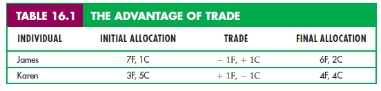
Suppose James and Karen have 10 units of food and 6 units of clothing between them. Table 16.1 shows that initially James has 7 units of food and 1 unit of clothing, and Karen 3 units of food and 5 units of clothing. To decide whether a trade would be advantageous, we need to know their preferences for food and clothing. Suppose that because Karen has a lot of clothing and little food, her marginal rate of substitution (MRS) of food for clothing is 3: To get 1 unit of food, she will give up 3 units of clothing. However, James’s MRS of food for clothing is only 1/2: He will give up only 1/2 a unit of clothing to get 1 unit of food.
There is thus room for mutually advantageous trade because James values clothing more highly than Karen does, whereas Karen values food more highly than James does. To get another unit of food, Karen would be willing to trade up to 3 units of clothing. But James will give up 1 unit of food for 1/2 unit of cloth- ing. The actual terms of the trade depend on the bargaining process. Among the possible outcomes are a trade of 1 unit of food by James for anywhere between 1/2 and 3 units of clothing from Karen.
Suppose Karen offers James 1 unit of clothing for 1 unit of food, and James agrees. Both will be better off. James will have more clothing, which he values more than food, and Karen will have more food, which she values more than clothing. Whenever two consumers’ MRSs are different, there is room for mutu-ally beneficial trade because the allocation of resources is inefficient: Trading will make both consumers better off. Conversely, to achieve economic efficiency, the two consumers’ MRSs must be equal.
This important result also holds when there are many goods and consumers:
An allocation of goods is efficient only if the goods are distributed so that the marginal rate of substitution between any pair of goods is the same for all consumers.
2. The Edgeworth Box Diagram
If trade is beneficial, which trades can occur? Which of those trades will allocate goods efficiently among customers? How much better off will consumers then be? We can answer these questions for any two-person, two-good example by using a diagram called an Edgeworth box.
Figure 16.4 shows an Edgeworth box in which the horizontal axis describes the number of units of food and the vertical axis the units of clothing. The length of the box is 10 units of food, the total quantity of food available; its height is 6 units of clothing, the total quantity of clothing available.
In the Edgeworth box, each point describes the market baskets of both con- sumers. James’s holdings are read from the origin at OJ and Karen’s holdings in the reverse direction from the origin at OK. For example, point A represents the initial allocation of food and clothing. Reading on the horizontal axis from left to right at the bottom of the box, we see that James has 7 units of food; reading upward along the vertical axis on the left of the diagram, we see that he has 1 unit of clothing. For James, therefore, A represents 7F and 1C. This leaves 3F and 5C for Karen. Karen’s allocation of food (3F) is read from right to left at the top of the box diagram beginning at OK; we read her allocation of clothing (5C) from top to bottom at the right of the box diagram.
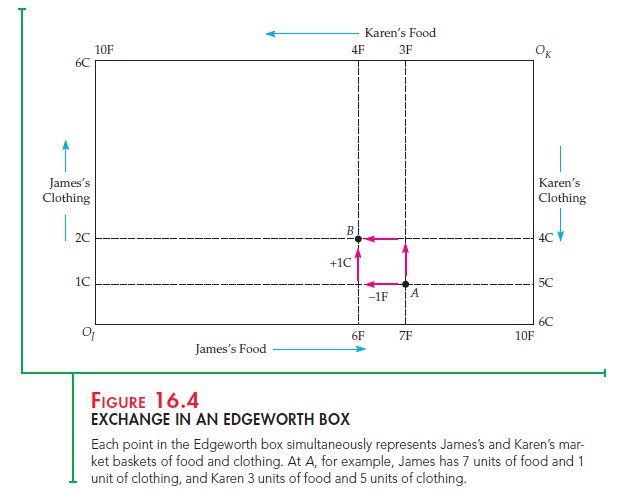
We can also see the effect of trade between Karen and James. James gives up 1F in exchange for 1C, moving from A to B. Karen gives up 1C and obtains 1F, also moving from A to B. Point B thus represents the market baskets of both James and Karen after the mutually beneficial trade.
3. Efficient Allocations
A trade from A to B thus made both Karen and James better off. But is B an efficient allocation? The answer depends on whether James’s and Karen’s MRSs are the same at B, which depends in turn on the shape of their indifference curves. Figure 16.5 shows several indifference curves for both James and Karen. Because his allocations are measured from the origin OJ, James’s indifference curves are drawn in the usual way. But for Karen, we have rotated the indiffer-ence curves 180 degrees, so that the origin is at the upper right-hand corner of the box. Karen’s indifference curves are convex, just like James’s; we simply see them from a different perspective.
Now that we are familiar with the two sets of indifference curves, let’s examine the curves labeled U} and UK that pass through the initial allocation at A. Both James’s and Karen’s MRSs give the slope of their indifference curves at A. James’s MRS of clothing for food is equal to 1/2, while Karen’s is 3. The shaded area between these two indifference curves represents all possible allocations of food and clothing that would make both James and Karen better off than at A. In other words, it describes all possible mutually beneficial trades.
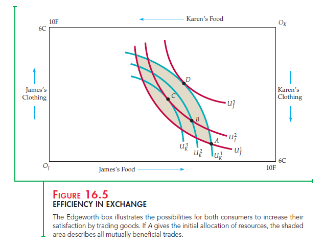 Starting at A, any trade that moved the allocation of goods outside the shaded area would make one of the two consumers worse off and should not occur. The move from A to B was mutually beneficial. But in Figure 16.5, B is not an efficient point because indifference curves U and UK intersect. In this case, James’s and Karen’s MRSs are not the same and the allocation is not efficient. Starting at B, James would prefer to give up some food to obtain additional clothing. He would be willing to make any trade that left him no worse off and hopefully gave him some additional utility, and there are many trades that would do so. Karen, on the other hand, would be willing to give up some clothing to obtain more food, and there are many such trades that would make her better off. This situation illustrates an important point: Even if a trade from an inefficient allocation makes both people better off, the new allocation is not necessarily efficient.
Suppose that from B the additional trade is made, with James giving up another unit of food to obtain another unit of clothing and Karen giving up a unit of clothing for a unit of food. Point C in Figure 16.5 gives the new allocation. At C, the MRSs of both people are identical, because at point C the indifference curves are tangent. Trading food for clothing and thereby moving from point B to point C has allowed James and Karen to achieve a Pareto efficient outcome, and they will both be better off. When the indifference curves are tangent, one person cannot be made better off without making the other person worse off. Therefore, C represents an efficient allocation.
Of course, C is not the only possible efficient outcome of a bargain between James and Karen. For example, if James is an effective bargainer, a trade might change the allocation of goods from A to D, where indifference curve Uf is tangent to indifference curve U 1 . This allocation would leave Karen no worse off than she was at A and James much better off. And because no further trade is possible, D is an efficient allocation. Thus C and D are both efficient alloca- tions, although James prefers D to C and Karen C to D. In general, it is difficult to predict the allocation that will be reached in a bargain because the end result depends on the bargaining abilities of the people involved.
4. The Contract Curve
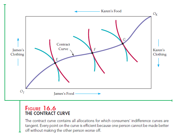
We have seen that from an initial allocation many possible efficient allocations can be reached through mutually beneficial trade. To find all possible efficient allo- cations of food and clothing between Karen and James, we look for all points of tangency between each of their indifference curves. Figure 16.6 shows the contract curve: the curve drawn through all such efficient allocations.
The contract curve shows all allocations from which no mutually beneficial trade can be made. These allocations are efficient because there is no way to reallocate goods to make someone better off without making someone else worse off. In Figure 16.5 three allocations labeled E, F, and G are Pareto efficient, although each involves a different distribution of food and clothing, because one person could not be made better off without making someone else worse off.
Several properties of the contract curve may help us understand the concept of efficiency in exchange. Once a point on a contract curve, such as E, has been chosen, there is no way to move to another point on the contract curve, say F, without making one person worse off (in this case, Karen). Karen is worse off because she has less food and less clothing at F than she had at E. Without mak- ing further comparison between James’s and Karen’s preferences, we cannot compare allocations E and F. We simply know that both are efficient. In this sense, Pareto efficiency is a modest goal: It says that we should make all mutu- ally beneficial exchanges, but it does not say which exchanges are best. Pareto efficiency can be a powerful concept, however. If a change will improve effi- ciency, it is in everyone’s self-interest to support it.
We can frequently improve efficiency even when one aspect of a proposed change makes someone worse off. We need only include a second change, such that the combined set of changes leaves someone better off and no one worse off. Suppose, for example, that we eliminate the quota on steel imports into the United States. Although U.S. consumers would then enjoy lower prices and a greater selection of cars, some U.S. workers would lose their jobs. But what if eliminating the quota were combined with federal tax breaks and job relocation subsidies for steelworkers? In that case, U.S. consumers would be better off (after accounting for the cost of the job subsidies) and the workers no worse off. This would increase efficiency.
5. Consumer Equilibrium in a Competitive Market
In a two-person exchange, the outcome can depend on the bargaining power of the two parties. Competitive markets, however, have many actual or potential buyers and sellers. As a result, each buyer and seller takes the price of the goods as fixed and decides how much to buy and sell at those prices. We can show how competitive markets lead to efficient exchange by using the Edgeworth box to mimic a competitive market. Suppose, for example, that there are many Jameses and many Karens. This allows us to think of each individual James and Karen as a price taker, even though we are working with only a two-person box diagram.
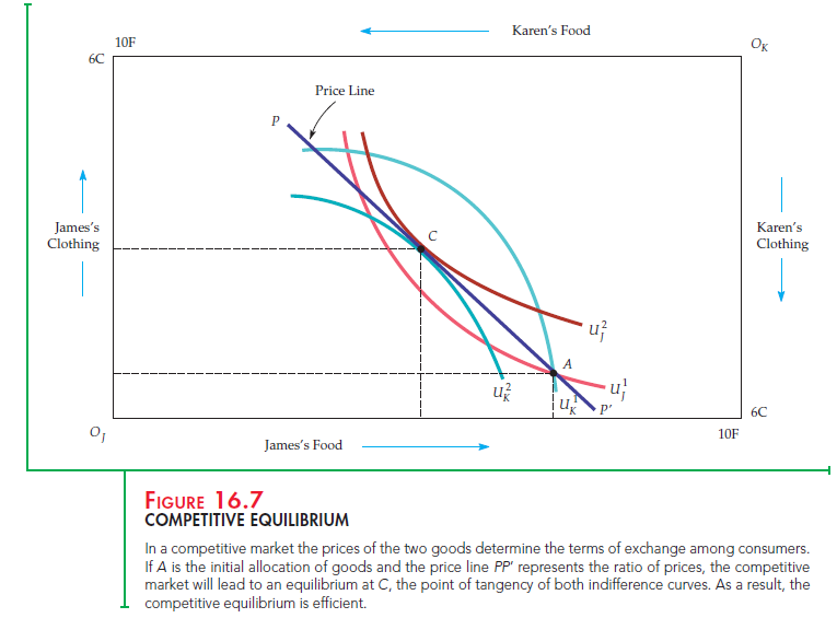
Figure 16.7 shows the opportunities for trade when we start at the allocation given by point A and when the prices of both food and clothing are equal to 1. (The actual prices do not matter; what matters is the price of food relative to the price of clothing.) When the prices of food and clothing are equal, each unit of food can be exchanged for 1 unit of clothing. As a result, the price line PP’ in the diagram, which has a slope of – 1, describes all possible allocations that exchange can achieve.
Suppose each James decides to buy 2 units of clothing and sell 2 units of food in exchange. This would move each James from A to C and increase satisfaction from indifference curve U} to Uj. Meanwhile, each Karen buys 2 units of food and sells 2 units of clothing. This would move each Karen from A to C as well, increasing satisfaction from indifference curve U1K to U2K.
We choose prices for the two goods so that the quantity of food demanded by each Karen is equal to the quantity of food that each James wishes to sell; likewise, the quantity of clothing demanded by each James is equal to the quantity of clothing that each Karen wishes to sell. As a result, the markets for food and clothing are in equilibrium. An equilibrium is a set of prices at which the quantity demanded equals the quantity supplied in every market. This is also a competitive equilibrium because all suppliers and demanders are price takers.
Not all prices are consistent with equilibrium. For example, if the price of food is 3 and the price of clothing is 1, any exchange of clothing for food must be done on a 3-to-1 basis, i.e., 3 units of clothing must be given up to obtain 1 unit of food. But then each James will be unwilling to trade any clothing to get additional food because his MRS of clothing for food is only 1/2, i.e., he would only be willing to give up 2 units of clothing for 1 unit of food. Each Karen, on the other hand, would be happy to sell clothing to get more food but has no one to trade with. The market is therefore in disequilibrium because the quantities of food and clothing demanded are not equal to the quantities supplied.
This disequilibrium should be only temporary. In a competitive market, prices will adjust if there is excess demand in some markets (the quantity demanded of one good is greater than the quantity supplied) and excess supply in others (the quantity supplied is greater than the quantity demanded). In our example, each Karen’s quantity demanded for food is greater than each James’s willingness to sell it, whereas each Karen’s willingness to trade clothing is greater than each James’s quantity demanded. As a result of this excess quantity demanded for food and excess quantity supplied of clothing, we can expect the price of food to increase relative to the price of clothing. As the price changes, so will the quanti- ties demanded by all those in the market. Eventually, the prices will adjust until an equilibrium is reached. In our example, the price of both food and clothing might be 2; we know from the previous analysis that when the price of cloth- ing is equal to the price of food, the market will be in competitive equilibrium. (Recall that only relative prices matter; prices of 2 for clothing and food are equivalent to prices of 1 for each.)
Note the important difference between exchange with two people and an economy with many people. When only two people are involved, bargaining leaves the outcome indeterminate. However, when many people are involved, the prices of the goods are determined by the combined choices of demanders and suppliers of goods.
6. The Economic Efficiency of Competitive Markets
We can now understand one of the fundamental results of microeconomic anal- ysis. We can see from point C in Figure 16.7 that the allocation in a competitive equilibrium is Pareto efficient. The key reason why this is so is that C must occur at the tangency of two indifference curves. If it does not, one of the Jameses or one of the Karens will not be achieving maximum satisfaction; he or she will be willing to trade to achieve a higher level of utility.
This result holds in an exchange framework and in a general equilibrium set- ting in which all markets are perfectly competitive. It is the most direct way of illustrating the workings of Adam Smith’s famous invisible hand, because it tells us that the economy will automatically allocate resources in a Pareto efficient manner without the need for regulatory control. It is the independent actions of consumers and producers, who take prices as given, that allows markets to function in an economically efficient manner. Not surprisingly, the invisi- ble-hand result is often used as the norm against which the workings of all real-world markets are compared. For some, the invisible hand supports the normative argument for less government intervention; they argue that markets are highly competitive. For others, the invisible hand supports a more expan- sive role for government; they reply that intervention is needed to make mar- kets more competitive.
Whatever one’s view of government intervention, most economists con- sider the invisible-hand result important. In fact, the result that a competitive equilibrium is Pareto efficient is often described as the first theorem of welfare economics, which involves the normative evaluation of markets and economic policy. Formally, the first theorem states the following:

Let’s summarize what we know about a competitive equilibrium from the consumer ’s perspective:
- Because the indifference curves are tangent, all marginal rates of substitu- tion between consumers are equal.
- Because each indifference curve is tangent to the price line, each person’s MRS of clothing for food is equal to the ratio of the prices of the two goods.
To be as clear as possible, we will use the notation MRSFC to denote the MRS of food for clothing. Then, if PC and PF are the two prices, competitive. But efficient outcomes can also be achieved by other means—for example, through a centralized system in which the government allocates all goods and services. The competitive solution is often preferred because it allo- cates resources with a minimum of information. All consumers must know their own preferences and the prices they face, but they need not know what is being produced or the demands of other consumers. Other allocation methods need more information, and as a result, they become difficult and cumbersome to manage.

Source: Pindyck Robert, Rubinfeld Daniel (2012), Microeconomics, Pearson, 8th edition.
Lovely just what I was searching for.Thanks to the author for taking his clock time on this one.