Revealed Preference

In Section 3.1, we saw how an individual’s preferences could be represented by a series of indifference curves. Then in Section 3.3, we saw how preferences, given budget constraints, determine choices. Can this process be reversed? If we know the choices that a consumer has made, can we determine his or her preferences?

We can if we have information about a sufficient number of choices that have been made when prices and income levels varied. The basic idea is simple. If a consumer chooses one market basket over another, and if the chosen market basket is more expensive than the alternative, then the consumer must pre- fer the chosen market basket.

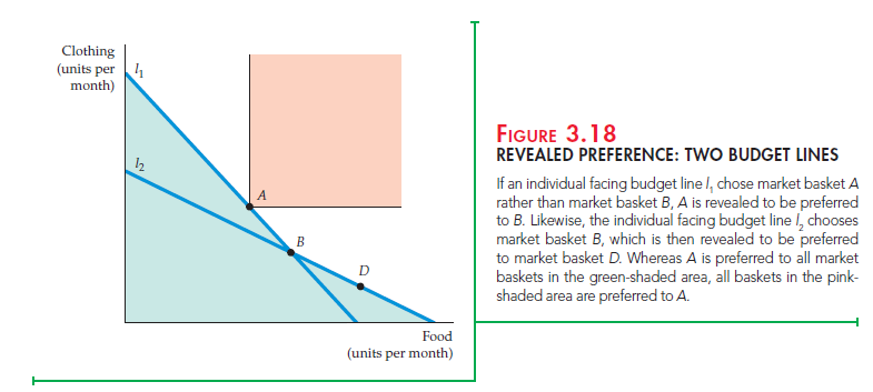
Suppose that an individual, facing the budget constraint given by line l1 in Figure 3.18, chooses market basket A. Let’s compare A to baskets B and D. Because the individual could have purchased basket B (and all baskets below line l1) and did not, we say that A is preferred to B.

It might seem at first glance that we cannot make a direct comparison between baskets A and D because D is not on l1. But suppose the relative prices of food and clothing change, so that the new budget line is l2  and the individual then chooses market basket B. Because D lies on budget line l2  and was not chosen, B is preferred to D (and to all baskets below line l2). Because A is preferred to B and B is preferred to D, we conclude that A is preferred to D. Furthermore, note in Figure 3.18 that basket A is preferred to all of the bas- kets that appear in the green-shaded areas. However, because food and cloth- ing are “goods” rather than “bads,” all baskets that lie in the pink-shaded area in the rectangle above and to the right of A are preferred to A. Thus, the indifference curve passing through A must lie in the unshaded area.

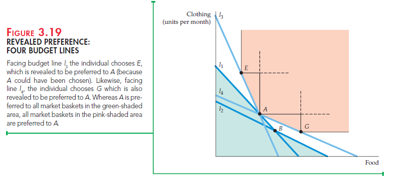
Given more information about choices when prices and income levels vary, we can get a better fix on the shape of the indifference curve. Consider Figure 3.18. Suppose that facing line l3  (which was chosen to pass through A), the individ- ual chooses market basket E. Because E was chosen even though A was equally expensive (it lies on the same budget line), E is preferred to A, as are all points in the rectangle above and to the right of E. Now suppose that facing line l4  (which passes through A), the individual chooses market basket G. Because G was cho- sen and A was not, G is preferred to A, as are all market baskets above and to the right of G.

We can go further by making use of the assumption that indifference curves are convex. In that case, because E is preferred to A, all market baskets above and to the right of line AE in Figure 3.19 must be preferred to A. Otherwise, the indifference curve passing through A would have to pass through a point above and to the right of AE and then fall below the line at E—in which case the indif- ference curve would not be convex. By a similar argument, all points on AG or above are also preferred to A. Therefore, the indifference curve must lie within the unshaded area.

The revealed preference approach is valuable as a means of checking whether individual choices are consistent with the assumptions of consumer theory. As Example 3.6 shows, revealed preference analysis can help us understand the implications of choices that consumers must make in particu- lar circumstances.

Source: Pindyck Robert, Rubinfeld Daniel (2012), Microeconomics, Pearson, 8th edition.