So far, our discussion of market power has focused entirely on the seller side of the market. Now we turn to the buyer side. We will see that if there are not too many buyers, they can also have market power and use it profitably to affect the price they pay for a product.
First, a few terms.
- Monopsony refers to a market in which there is a single buyer.
- An oligopsony is a market with only a few buyers.
- With one or only a few buyers, some buyers may have monopsony power: a buyer ’s ability to affect the price of a good. Monopsony power enables the buyer to purchase a good for less than the price that would prevail in a competitive market.
Suppose you are trying to decide how much of a good to purchase. You could apply the basic marginal principle—keep purchasing units of the good until the last unit purchased gives additional value, or utility, just equal to the cost of that last unit. In other words, on the margin, additional benefit should just be offset by additional cost.
Let’s look at this additional benefit and additional cost in more detail. We use the term marginal value to refer to the additional benefit from purchasing one more unit of a good. How do we determine marginal value? Recall from Chapter 4 that an individual demand curve determines marginal value, or mar- ginal utility, as a function of the quantity purchased. Therefore, your marginal value schedule is your demand curve for the good. An individual’s demand curve slopes downward because the marginal value obtained from buying one more unit of a good declines as the total quantity purchased increases.
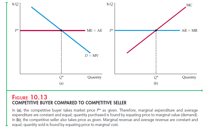
The additional cost of buying one more unit of a good is called the marginal expenditure. What that marginal expenditure is depends on whether you are a competitive buyer or a buyer with monopsony power. Suppose you are a competitive buyer—in other words, you have no influence over the price of the good. In that case, the cost of each unit you buy is the same no matter how many units you purchase; it is the market price of the good. Figure 10.13(a) illustrates this principle. The price you pay per unit is your average expenditure per unit, and it is the same for all units. But what is your marginal expenditure per unit? As a competitive buyer, your marginal expenditure is equal to your average expen- diture, which in turn is equal to the market price of the good.
Figure 10.13(a) also shows your marginal value schedule (i.e., your demand curve). How much of the good should you buy? You should buy until the mar- ginal value of the last unit is just equal to the marginal expenditure on that unit. Thus you should purchase quantity Q* at the intersection of the marginal expen- diture and demand curves.
We introduced the concepts of marginal and average expenditure because they will make it easier to understand what happens when buyers have mon- opsony power. But before considering that situation, let’s look at the anal- ogy between competitive buyer conditions and competitive seller conditions. Figure 10.13(b) shows how a perfectly competitive seller decides how much to produce and sell. Because the seller takes the market price as given, both aver- age and marginal revenue are equal to the price. The profit-maximizing quan- tity is at the intersection of the marginal revenue and marginal cost curves.
Now suppose that you are the only buyer of the good. Again you face a mar- ket supply curve, which tells you how much producers are willing to sell as a function of the price you pay. Should the quantity you purchase be at the point where your marginal value curve intersects the market supply curve? No. If you want to maximize your net benefit from purchasing the good, you should purchase a smaller quantity, which you will obtain at a lower price.
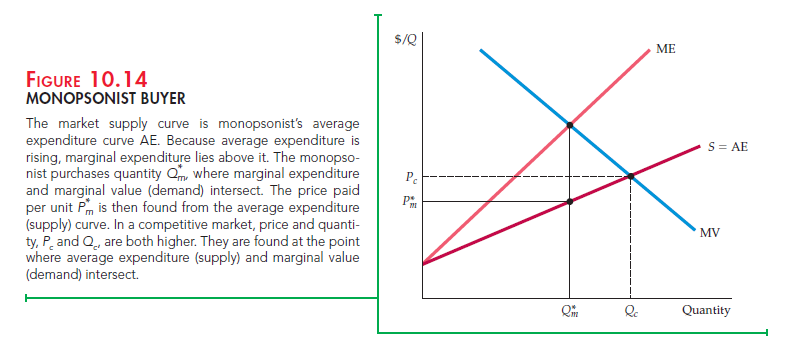
To determine how much to buy, set the marginal value from the last unit purchased equal to the marginal expenditure on that unit.14 Note, however, that the market supply curve is not the marginal expenditure curve. The mar- ket supply curve shows how much you must pay per unit, as a function of the total number of units you buy. In other words, the supply curve is the aver- age expenditure curve. And because this average expenditure curve is upward sloping, the marginal expenditure curve must lie above it. The decision to buy an extra unit raises the price that must be paid for all units, not just the extra one.15
Figure 10.14 illustrates this principle. The optimal quantity for the monopso- nist to buy, Q* , is found at the intersection of the demand and marginal expen-diture curves. The price that the monopsonist pays is found from the supply curve: It is the price Pm that brings forth the supply Qm. Finally, note that this quantity Qm is less, and the price Pm is lower, than the quantity and price that would prevail in a competitive market, Qc and Pc.
Monopsony and Monopoly Compared
Monopsony is easier to understand if you compare it with monopoly. Figures 10.15(a) and 10.15(b) illustrate this comparison. Recall that a monopo- list can charge a price above marginal cost because it faces a downward-sloping demand, or average revenue curve, so that marginal revenue is less than aver- age revenue. Equating marginal cost with marginal revenue leads to a quantity Q* that is less than what would be produced in a competitive market, and to a price P* that is higher than the competitive price Pc.
The monopsony situation is exactly analogous. As Figure 10.15(b) illus-trates, the monopsonist can purchase a good at a price below its marginal value because it faces an upward-sloping supply, or average expenditure, curve. Thus for a monopsonist, marginal expenditure is greater than average expenditure.
Equating marginal value with marginal expenditure leads to a quantity Q* that is less than what would be bought in a competitive market, and to a price P* that is lower than the competitive price Pc.
Source: Pindyck Robert, Rubinfeld Daniel (2012), Microeconomics, Pearson, 8th edition.
I was studying some of your posts on this site and I believe this internet site is rattling instructive! Continue posting.