We have seen that the demand for a good depends not only on its price, but also on consumer income and on the prices of other goods. Likewise, supply depends both on price and on variables that affect production cost. For example, if the price of coffee increases, the quantity demanded will fall and the quantity supplied will rise. Often, however, we want to know how much the quantity sup- plied or demanded will rise or fall. How sensitive is the demand for coffee to its price? If price increases by 10 percent, how much will the quantity demanded change? How much will it change if income rises by 5 percent? We use elasticities to answer questions like these.
An elasticity measures the sensitivity of one variable to another. Specifically, it is a number that tells us the percentage change that will occur in one variable in response to a 1-percent increase in another variable. For example, the price elasticity of demand measures the sensitivity of quantity demanded to price changes. It tells us what the percentage change in the quantity demanded for a good will be fol- lowing a 1-percent increase in the price of that good.
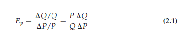
PRICE ELASTICITY OF DEMAND Let’s look at this in more detail. We write the price elasticity of demand, Ep, as
![]()
where % AQ means “percentage change in quantity demanded” and %AP means “percentage change in price.” (The symbol A is the Greek capital letter delta; it means “the change in.” So AX means “the change in the variable X,” say, from one year to the next.) The percentage change in a variable is just the absolute change in the variable divided by the original level of the variable. (If the Consumer Price Index were 200 at the beginning of the year and increased to 204 by the end of the year, the percentage change—or annual rate of inflation—would be 4/200 = .02, or 2 percent.) Thus we can also write the price elasticity of demand as follows:[1]
The price elasticity of demand is usually a negative number. When the price of a good increases, the quantity demanded usually falls. Thus AQ/ AP (the change in quantity for a change in price) is negative, as is E . Sometimes we refer to the magnitude of the price elasticity—i.e., its absolute size. For example, if Ep = – 2, we say that the elasticity is 2 in magnitude.
When the price elasticity is greater than 1 in magnitude, we say that demand is price elastic because the percentage decline in quantity demanded is greater than the percentage increase in price. If the price elasticity is less than 1 in magnitude, demand is said to be price inelastic. In general, the price elasticity of demand for a good depends on the availability of other goods that can be substituted for it. When there are close substitutes, a price increase will cause the consumer to buy less of the good and more of the substitute. Demand will then be highly price elastic. When there are no close substitutes, demand will tend to be price inelastic.
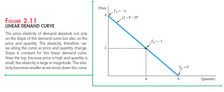
LINEAR DEMAND CURVE Equation (2.1) says that the price elasticity of demand is the change in quantity associated with a change in price (A Q/ A P) times the ratio of price to quantity (P/Q). But as we move down the demand curve, AQ/APmay change, and the price and quantity will always change. Therefore, the price elasticity of demand must be measured at a particular point on the demand curve and will generally change as we move along the curve.
This principle is easiest to see for a linear demand curve—that is, a demand curve of the form
Q = a – bP
As an example, consider the demand curve
Q = 8 – 2P
For this curve, AQ/AP is constant and equal to — 2 (a AP of 1 results in a AQ of —2). However, the curve does not have a constant elasticity. Observe from Figure 2.11 that as we move down the curve, the ratio P/Q falls; the elasticity therefore decreases in magnitude. Near the intersection of the curve with the price axis, Q is very small, so Ep = — 2(P/Q) is large in magnitude. When P = 2 and Q = 4 , Ep = — 1. At the intersection with the quantity axis, P = 0 so EP = 0.
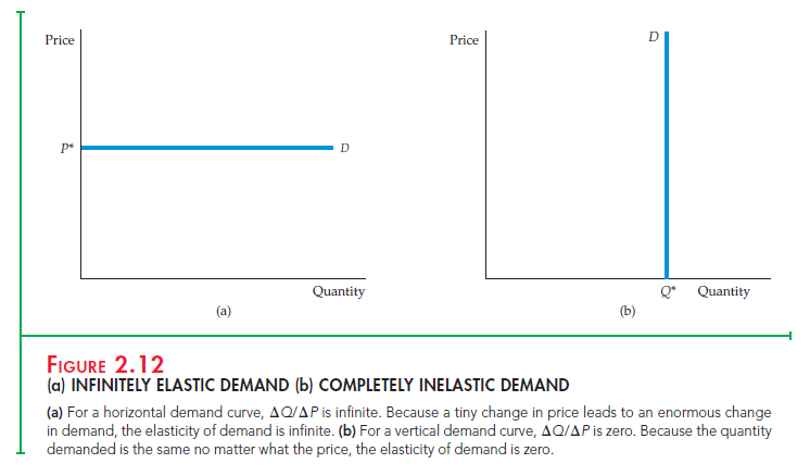
Because we draw demand (and supply) curves with price on the vertical axis and quantity on the horizontal axis, AQ/AP = (1/slope of curve). As a result, for any price and quantity combination, the steeper the slope of the curve, the less elastic is demand. Figure 2.12 shows two special cases. Figure 2.12(a) shows a demand curve reflecting infinitely elastic demand: Consumers will buy as much as they can at a single price P*. For even the smallest increase in price above this level, quantity demanded drops to zero, and for any decrease in price, quantity demanded increases without limit. The demand curve in Figure 2.12(b), on the other hand, reflects completely inelastic demand: Consumers will buy a fixed quantity Q*, no matter what the price.
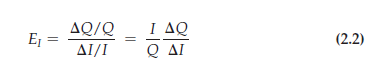
OTHER DEMAND ELASTICITIES We will also be interested in elasticities of demand with respect to other variables besides price. For example, demand for most goods usually rises when aggregate income rises. The income elasticity of demand is the percentage change in the quantity demanded, Q, resulting from a 1-percent increase in income I:
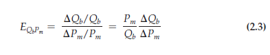
The demand for some goods is also affected by the prices of other goods. For example, because butter and margarine can easily be substituted for each other, the demand for each depends on the price of the other. A cross-price elasticity of demand refers to the percentage change in the quantity demanded for a good that results from a 1-percent increase in the price of another good. So the elasticity of demand for butter with respect to the price of margarine would be written as
The demand for some goods is also affected by the prices of other goods. For example, because butter and margarine can easily be substituted for each other, the demand for each depends on the price of the other. A cross-price elasticity of demand refers to the percentage change in the quantity demanded for a good that results from a 1-percent increase in the price of another good. So the elasticity of demand for butter with respect to the price of margarine would be written as where Qb is the quantity of butter and Pm is the price of margarine.
gasoline demanded falls—motorists will drive less. And because people are driving less, the demand for motor oil also falls. (The entire demand curve for motor oil shifts to the left.) Thus, the cross-price elasticity of motor oil with respect to gasoline is negative.
ELASTICITIES OF SUPPLY Elasticities of supply are defined in a similar manner. The price elasticity of supply is the percentage change in the quantity supplied resulting from a 1-percent increase in price. This elasticity is usually positive because a higher price gives producers an incentive to increase output.
We can also refer to elasticities of supply with respect to such variables as interest rates, wage rates, and the prices of raw materials and other intermediate goods used to manufacture the product in question. For example, for most manufactured goods, the elasticities of supply with respect to the prices of raw materials are negative. An increase in the price of a raw material input means higher costs for the firm; other things being equal, therefore, the quantity supplied will fall.
Point versus Arc Elasticities
So far, we have considered elasticities at a particular point on the demand curve or the supply curve. These are called point elasticities. The point elasticity of demand, for example, is the price elasticity of demand at a particular point on the demand curve and is defined by Equation (2.1). As we demonstrated in Figure 2.11 using a linear demand curve, the point elasticity of demand can vary depending on where it is measured along the demand curve.
There are times, however, when we want to calculate a price elasticity over some portion of the demand curve (or supply curve) rather than at a single point. Suppose, for example, that we are contemplating an increase in the price of a product from $8.00 to $10.00 and expect the quantity demanded to fall from 6 units to 4. How should we calculate the price elasticity of demand? Is the price increase 25 percent (a $2 increase divided by the original price of $8), or is it 20 percent (a $2 increase divided by the new price of $10)? Is the percentage decrease in quantity demanded 33 1/3 percent (2/6) or 50 percent (2/4)?
There is no correct answer to such questions. We could calculate the price elasticity using the original price and quantity. If so, we would find that Ep = (- 33 1/3 percent/25 percent) = -1.33. Or we could use the new price and quantity, in which case we would find that Ep = (- 50 percent/20 percent) = – 2.5. The difference between these two calculated elastici ties is large, and neither seems preferable to the other.
ARC ELASTICITY OF DEMAND We can resolve this problem by using the arc elasticity of demand: the elasticity calculated over a range of prices. Rather than choose either the initial or the final price, we use an average of the two, P; for the quantity demanded, we use Q. Thus the arc elasticity of demand is given by Arc elasticity: ![]()
In our example, the average price is $9 and the average quantity 5 units. Thus the arc elasticity is
Ep = ( – 2/$2)($9/5) = -1.8
The arc elasticity will always lie somewhere (but not necessarily halfway) between the point elasticities calculated at the lower and the higher prices.
Although the arc elasticity of demand is sometimes useful, economists generally use the word “elasticity” to refer to a point elasticity. Throughout the rest of this book, we will do the same, unless noted otherwise.
Source: Pindyck Robert, Rubinfeld Daniel (2012), Microeconomics, Pearson, 8th edition.
Way cool, some valid points! I appreciate you making this article available, the rest of the site is also high quality. Have a fun.