Sequential Games

In most of the games we have discussed so far, both players move at the same time. In the Cournot model of duopoly, for example, both firms set output at the same time. In sequential games, players move in turn. The Stackelberg model discussed in Chapter 12 is an example of a sequential game; one firm sets output before the other does. There are many other examples: an advertising decision by one firm and the response by its competitor; entry-deterring investment by an incumbent firm and the decision whether to enter the market by a potential competitor; or a new government regulatory policy and the investment and out­put response of the regulated firms.

We will look at a variety of sequential games in the remainder of this chapter. As we will see, they are often easier to analyze than games in which the players move at the same time. In a sequential game, the key is to think through the pos­sible actions and rational reactions of each player.

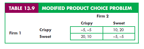
As a simple example, let’s return to the product choice problem first dis­cussed in Section 13.3. This problem involves two companies facing a market in which two new variations of breakfast cereal can be successfully introduced as long as each firm introduces only one variation. This time, let’s change the payoff matrix slightly. As Table 13.9 shows, the new sweet cereal will inevitably be a better seller than the new crispy cereal, earning a profit of 20 rather than 10 (perhaps because consumers prefer sweet things to crispy things). Both new cereals will still be profitable, however, as long as each is introduced by only one firm. (Compare Table 13.9 with Table 13.3—page 493.)

Suppose that both firms, in ignorance of each other’s intentions, must announce their decisions independently and simultaneously. In that case, both will probably introduce the sweet cereal—and both will lose money.

Now suppose that Firm 1 can gear up its production faster and introduce its new cereal first. We now have a sequential game: Firm 1 introduces a new cereal, and then Firm 2 introduces one. What will be the outcome of this game? When making its decision, Firm 1 must consider the rational response of its competi­tor. It knows that whichever cereal it introduces, Firm 2 will introduce the other kind. Thus it will introduce the sweet cereal, knowing that Firm 2 will respond by introducing the crispy one.

1. The Extensive Form of a Game

Although this outcome can be deduced from the payoff matrix in Table 13.9, sequential games are sometimes easier to visualize if we represent the pos- sible moves in the form of a decision tree. This representation is called the extensive form of a game and is shown in Figure 13.2. The figure shows the possible choices of Firm 1 (introduce a crispy or a sweet cereal) and the pos- sible responses of Firm 2 to each of those choices. The resulting payoffs are given at the end of each branch. For example, if Firm 1 produces a crispy cereal and Firm 2 responds by also producing a crispy cereal, each firm will have a payoff of – 5.

To find the solution to the extensive form game, work backward from the end. For Firm 1, the best sequence of moves is the one in which it earns 20 and Firm 2 earns 10. Thus it can deduce that it should produce the sweet cereal because Firm 2’s best response is then to produce the crispy cereal.

2. The Advantage of Moving First

In this product-choice game, there is a clear advantage to moving first: By introducing the sweet cereal, Firm 1 leaves Firm 2 little choice but to introduce the crispy one. This is much like the first-mover advantage that we saw in the Stackelberg model in Chapter 12. In that model, the firm that moves first can choose a large level of output, thereby giving its competitor little choice but to choose a small level.

To clarify the nature of this first-mover advantage, it will be useful to review the Stackelberg model and compare it to the Cournot model in which both firms choose their outputs simultaneously. As in Chapter 12, we will use the example in which two duopolists face the market demand curve

P = 30 – Q

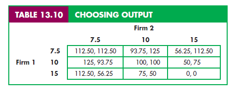
where Q is the total production, i.e., Q = Q₁ + Q₂. As before, we will also assume that both firms have zero marginal cost. Recall that the Cournot equilibrium is then Q₁ = Q₂ = 10, so that P = 10 and each firm earns a profit of 100. Recall also that if the two firms colluded, they would set Q₁ = Q₂ = 7.5, so that P = 15 and each firm earns a profit of 112.50. Finally, recall from Section 12.3 that in the Stackelberg model, in which Firm 1 moves first, the outcome is Q₁ = 15 and Q₂ = 7.5, so that P = 7.50 and the firms’ profits are 112.50 and 56.25, respectively.

These and a few other possible outcomes are summarized in the payoff matrix in Table 13.10. If both firms move simultaneously, the only solution to the game is that both produce 10 and earn 100. In this Cournot equilibrium each firm is doing the best it can given what its competitor is doing. If Firm 1 moves first, however, it knows that its decision will constrain Firm 2’s choice. Observe from the payoff matrix that if Firm 1 sets Q₁ = 7.5, Firm 2’s best response will be to set Q₂ = 10. This will give Firm 1 a profit of 93.75 and Firm 2 a profit of 125. If Firm 1 sets Q₁ = 10, Firm 2 will set Q₂ = 10, and both firms will earn 100. But if Firm 1 sets Q₁ = 15, Firm 2 will set Q₂ = 7.5, so that Firm 1 earns 112.50, and Firm 2 earns 56.25. Therefore, the most that Firm 1 can earn is 112.50, and it does so by setting Q₁ = 15. Compared to the Cournot outcome, when Firm 1 moves first, it does better—and Firm 2 does much worse.

Source: Pindyck Robert, Rubinfeld Daniel (2012), Microeconomics, Pearson, 8th edition.