Dynamic Changes in Costs—The Learning Curve

Our discussion thus far has suggested one reason why a large firm may have a lower long-run average cost than a small firm: increasing returns to scale in production. It is tempting to conclude that firms that enjoy lower average cost over time are growing firms with increasing returns to scale. But this need not be true. In some firms, long-run average cost may decline over time because workers and managers absorb new technological information as they become more experienced at their jobs.

As management and labor gain experience with production, the firm’s marginal and average costs of producing a given level of output fall for four reasons:

1. Workers often take longer to accomplish a given task the first few times they do it. As they become more adept, their speed increases.
2. Managers learn to schedule the production process more effectively, from the flow of materials to the organization of the manufacturing itself.
3. Engineers who are initially cautious in their product designs may gain enough experience to be able to allow for tolerances in design that save costs without increasing defects. Better and more specialized tools and plant organization may also lower cost.
4. Suppliers may learn how to process required materials more effectively and pass on some of this advantage in the form of lower costs.

As a consequence, a firm “learns” over time as cumulative output increases. Managers can use this learning process to help plan production and forecast future costs. Figure 7.11 illustrates this process in the form of a learning curve—a curve that describes the relationship between a firm’s cumulative output and the amount of inputs needed to produce each unit of output.

1. Graphing the Learning Curve

Figure 7.12 shows a learning curve for the production of machine tools. The horizontal axis measures the cumulative number of lots of machine tools (groups of approximately 40) that the firm has produced. The vertical axis shows the number of hours of labor needed to produce each lot. Labor input per unit of output directly affects the production cost because the fewer the hours of labor needed, the lower the marginal and average cost of production.

The learning curve in Figure 7.12 is based on the relationship

where N is the cumulative units of output produced and L the labor input per unit of output. A, B, and b are constants, with A and B positive, and b between 0 and 1. When N is equal to 1, L is equal to A + B, so that A + B measures the labor input required to produce the first unit of output. When b equals 0, labor input per unit of output remains the same as the cumulative level of output increases; there is no learning. When b is positive and N gets larger and larger, L becomes arbitrarily close to A. A, therefore, represents the minimum labor input per unit of output after all learning has taken place.

The larger b is, the more important the learning effect. With b equal to 0.5, for example, the labor input per unit of output falls proportionately to the square root of the cumulative output. This degree of learning can substantially reduce production costs as a firm becomes more experienced.

In this machine tool example, the value of b is 0.31. For this particular learning curve, every doubling in cumulative output causes the input requirement (less the minimum attainable input requirement) to fall by about 20 percent.¹² As Figure 7.12 shows, the learning curve drops sharply as the cumulative number of lots increases to about 20. Beyond an output of 20 lots, the cost savings are relatively small.

2. Learning versus Economies of Scale

Once the firm has produced 20 or more machine lots, the entire effect of the learning curve would be complete, and we could use the usual analysis of cost. If, however, the production process were relatively new, relatively high cost at low levels of output (and relatively low cost at higher levels) would indicate learning effects, not economies of scale. With learning, the cost of pro- duction for a mature firm is relatively low regardless of the scale of the firm’s operation. If a firm that produces machine tools in lots knows that it enjoys economies of scale, it should produce its machines in very large lots to take advantage of the lower cost associated with size. If there is a learning curve, the firm can lower its cost by scheduling the production of many lots regard­less of individual lot size.

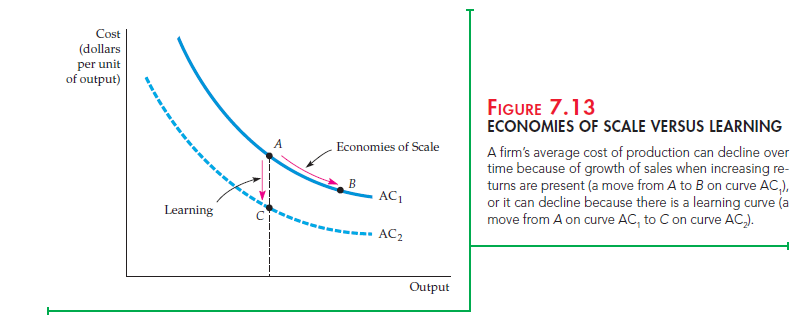
Figure 7.13 shows this phenomenon. AC_X represents the long-run average cost of production of a firm that enjoys economies of scale in production. Thus the increase in the rate of output from A to B along AC₁ leads to lower cost due to economies of scale. However, the move from A on AC₁ to C on AC₂ leads to lower cost due to learning, which shifts the average cost curve downward.

The learning curve is crucial for a firm that wants to predict the cost of produc­ing a new product. Suppose, for example, that a firm producing machine tools knows that its labor requirement per machine for the first 10 machines is 1.0, the minimum labor requirement A is equal to zero, and b is approximately equal to 0.32. Table 7.3 calculates the total labor requirement for producing 80 machines.

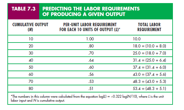
Because there is a learning curve, the per-unit labor requirement falls with increased production. As a result, the total labor requirement for producing more and more output increases in smaller and smaller increments. Therefore, a firm looking only at the high initial labor requirement will obtain an overly pessimistic view of the business. Suppose the firm plans to be in business for a long time, producing 10 units per year. Suppose the total labor require- ment for the first year ’s production is 10. In the first year of production, the firm’s cost will be high as it learns the business. But once the learning effect has taken place, production costs will fall. After 8 years, the labor required to produce 10 units will be only 5.1, and per-unit cost will be roughly half what it was in the first year of production. Thus, the learning curve can be important for a firm deciding whether it is profitable to enter an industry.

Source: Pindyck Robert, Rubinfeld Daniel (2012), Microeconomics, Pearson, 8th edition.