Generating and Replacing Variables in Stata

The generate and replace commands allow us to create new variables or change the values of existing variables. For example, in Canada, as in most industrial societies, women tend to live longer than men. To analyze regional variations in this gender gap, we might retrieve dataset Canadal.dta and generate a new variable equal to female life expectancy (flife) minus male life expectancy (mlife). In the main part of a generate or replace statement (unlike if qualifiers) we use a single equals sign.

For the province of Newfoundland, the true value of gap should be 79.8 – 73.9 = 5.9 years, but the output shows this value as 5.900002 instead. Like all computer programs, Stata stores numbers in binary form, and 5.9 has no exact binary representation. The small inaccuracies that arise from approximating decimal fractions in binary are unlikely to affect statistical calculations much, but they appear disconcerting in data lists. We can change the display format so that Stata shows only a rounded-off version. The following command specifies a fixed display format four numerals wide, with one digit to the right of the decimal:

. format gap %4.1f

Even when the display shows 5.9, however, a command such as the following will return no observations:

. list if gap == 5.9

This occurs because Stata believes the value does not exactly equal 5.9. (More technically, Stata stores gap values in single, float precision but does all calculations in double precision, and the single- and double-precision approximations of 5.9 are not identical.)

Display formats, as well as variables names and labels, can also be changed by double-clicking on a column in the Data Editor. Fixed numeric formats such as %4.1f are one of the three most common numeric display format types. These are

°%w.dg     General numeric format, where w specifies the total width or number of columns displayed and d the minimum number of digits that must follow the decimal point. Exponential notation (such as 1.00e+07, meaning 1.00 x 10⁷ or 10 million) and shifts in the decimal-point position will be used automatically as needed, to display values in an optimal (but varying) fashion.

%w.df       Fixed numeric format, where w specifies the total width or number of columns displayed and d the fixed number of digits that must follow the decimal point.

%w.de        Exponential numeric format, where w specifes the total width or number of columns displayed and d the fixed number of digits that must follow the decimal point.

For example, as we saw in Table 2.1, the 1995 population of Canada was approximately 29,606,100 people, and the Yukon Territory population was 30,100. The table below shows how those two numbers appear under several different display formats.

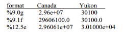
Although the displayed values look different, their internal values are identical. Calculations remain unaffected by display formats. Other numeric display formatting options include the use of commas, left- and right-justification, or leading zeros. There also exist special formats for dates, time series variables and string variables. Type help format for more information.

replace can make the same sorts of calculations as generate, but it changes values of an existing variable instead of creating a new variable. For example, suppose that we had data on income in dollars. We decide it would be more convenient to work with income in thousands of dollars. To convert dollars to thousands of dollars, we divide all values by 1,000:

. replace income = income/1000

replace can make such wholesale changes, or it can be used with in or if qualifiers to selectively edit the data. Suppose our survey variables include age and year born. A command such as the following would correct one or more typos where a subject’s age had been incorrectly typed as 299 instead of 29:

. replace age = 29 if age = = 299

Alternatively, the following command could correct an error in the value of age for observation number 1453:

. replace age = 29 in 1453

For a more complicated example,

. replace age = 2012-,born if missing(age) | age+1 < 2012-born

This replaces values of variable age with 2012 minus the year of birth (born) if age is missing or if the reported age (plus one year) is less than 2012 minus the year of birth.

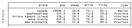
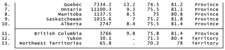
generate and replace provide tools to create categorical variables as well. We noted earlier that our Canadian dataset includes several types of observations: 2 territories, 10 provinces and one country combining them all. Although in and if qualifiers allow us to separate these, and drop can eliminate observations from the data, it might be most convenient to have a categorical variable that indicates the observation’s type. The following example shows one way to create such a variable, using our Canadal.dta dataset. We start by generating type as a constant, equal to 1 for each observation. Next, we replace this with the value 2 for the Yukon and Northwest Territories, and with 3 for Canada. The final steps involve labeling new variable type and defining labels for values 1, 2 and 3.

. use C:\data\Canada1, clear . generate type = 1

. replace type = 2 if place == “Yukon” | place = = “Northwest Territories”

. replace type = 3 if place == “Canada”

. label variable type “Province, territory or nation”

. label define typelbl 1 “Province” 2 “Territory” 3 “Nation”

. label values type typelbl

. list

As illustrated, labeling the values of a categorical variable requires two commands. The label define command specifies what labels go with what numbers. The label values command specifies to which variable these labels apply. One set of labels (created through one label define command) can apply to any number of variables (that is, be referenced in any number of label values commands). Value labels can have up to 32,000 characters, but work best for most purposes if they are not too long.

generate can create new variables, and replace can produce new values, using any mixture of old variables, constants, random values and expressions. For numeric variables, the following arithmetic operators apply:

+ add

– subtract

* multiply

/ divide

^ raise to power

Parentheses will control the order of calculation. Without them, the ordinary rules of precedence apply. Of the arithmetic operators, only addition, “+”, works with string variables, where it connects two string values into one.

Although their purposes differ, generate and replace have similar syntax. Either can use any mathematically or logically feasible combination of Stata operators and in or if qualifiers. These commands can also employ Stata’s broad array of special functions, introduced later.

Source: Hamilton Lawrence C. (2012), Statistics with STATA: Version 12, Cengage Learning; 8th edition.