Normality Tests and Transformations by using Stata

Many statistical procedures work best when applied to variables that follow normal distributions. The preceding section described exploratory methods to check for approximate normality, extending the graphical tools (histograms, box plots, symmetry plots and quantile-normal plots) presented in Chapter 3. A skewness-kurtosis test, making use of the skewness and kurtosis statistics shown by summarize, detail, can more formally evaluate the null hypothesis that the sample at hand came from a normally-distributed population.

sktest here rejects normality: elcap appears significantly nonnormal in skewness (p = .0223), although not in kurtosis (p = .0723), and in both statistics considered jointly (p = .0236).

Other normality tests include Shapiro-Wilk W (swilk) and Shapiro-Francia W’ (sfrancia) methods (type help sktest). A Stata module to perform Doornik-Hansen omnibus tests for univariate/multivariate normality is available online (type findit omninorm).

Nonlinear transformations such as square roots and logarithms are often employed to change distributions’ shapes, with the aim of making skewed distributions more symmetrical and perhaps more nearly normal. Transformations might also help linearize relationships between variables (Chapters 7 and 8). Table 5.1 shows a progression called the ladder of powers (Tukey 1977) that provides guidance for choosing transformations to change distributional shape. The variable lived exhibits mild positive skew, so its square root might be more symmetrical. We could create a new variable equal to the square root of elcap by typing

. generate srelcap = elcap ^.5

Instead of elcap ^.5, we could equally well have written sqrt(elcap).

Logarithms are another transformation that can reduce positive skew. To generate a new variable equal to the natural (base e) logarithm of elcap, type

. generate logelcap = ln(elcap)

In the ladder of powers and related transformation schemes such as Box-Cox, logarithms take the place of a “0” power. Their effect on distribution shape is intermediate between .5 (square root) and -.5 (reciprocal root) transformations.

We take negatives of the result after raising to a power less than zero, to preserve the original order — the highest value of old becomes transformed into the highest value of new, and so forth. When old itself contains negative or zero values, it is necessary to add a constant before
transformation. For example, if arrests measures the number of times a person has been arrested (0 for many people), then a suitable log transformation could be

. generate logarrest = ln(arrests + 1)

The ladder command combines the ladder of powers with sktest for normality. It tries each power on the ladder, and reports whether the result is significantly nonnormal. This can be illustrated using the positively skewed variable elcap, per capita electricity consumption, from electricity.dta.

Square root, log, inverse square root and inverse transformations all yield distributions that are not significantly different from normal. In this respect they offer improvements compared with the raw data or identity transformation, with is significantly nonnormal (p = .024). It appears that logarithms offer the best choice for a normalizing transformation. Figure 5.1, produced by the gladder command, visually supports this conclusion by comparing histograms of each transformation to normal curves.

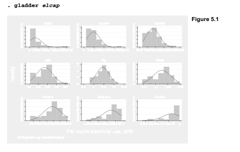
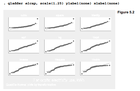
Figure 5.2 shows a corresponding set of quantile–normal plots for these ladder of powers transformations, obtained by thequantile ladder command qladder. (Type help ladder for information about ladder, gladder and qladder.) To make the tiny plots more readable in the example below, we scale the labels and marker symbols up by 25% with the scale(1.25) option. The axis labels (which would be unreadable and crowded) are suppressed by the options ylabel(none) xlabel(none)

An alternative technique called Box-Cox transformation offers finer gradations between transformations and automates the choice among them (easier for the analyst, but not always a good thing). The command bcskewO finds a value of X (lambda) for the transformations

such that y^(λ) has approximately zero skewness. Applying this to elcap, we obtain the transformed variable belcap:

That is, belcap = (elcap ¹⁴⁵ – 1)/(.145) is the transformation that comes closest to symmetry, as defined by the skewness statistic. The Box-Cox parameter X = .145 is not far from our ladder- of-powers choice, logarithms (which take the place of the 0 power). The confidence interval for X includes 0 (logarithm) but not 1 (identity or no change):

-.827 < λ < .878

Chapter 8 describes a Box-Cox approach to regression modeling.

Source: Hamilton Lawrence C. (2012), Statistics with STATA: Version 12, Cengage Learning; 8th edition.