Correlograms by using Stata

Autocorrelation coefficients estimate the correlation between a variable and itself at particular lags. For example, first-order autocorrelation is the correlation between y _t and y _t-1 . Second order refers to Cor[ yt,y _t-2], and so forth. A correlogram graphs correlation versus lag.

Stata’s corrgram command provides simple correlograms and related information. The maximum number of lags it shows can be limited by the data, by matsize, or to some arbitrary lower number that is set by specifying the lags( ) option:

Lags appear at the left side of the table, followed by columns of autocorrelations (AC) and partial autocorrelations (PAC). For example, the correlation between mei_t and mei_;_₂ is .8582, and the partial autocorrelation (adjusted for lag 1) is -.4181. The Q statistics (Ljung-Box portmanteau) test a series of null hypotheses that all autocorrelations up to and including a given lag are zero. Because the p-values seen here are all very small, we should reject the null hypotheses and conclude that the Multivariate ENSO Index (mei) exhibits significant autocorrelation. If none of the Q statistic probabilities had been below .05, we might conclude instead that the series was white noise with no significant autocorrelation.

At right in a corrgram output table are character-based plots of autocorrelations and partial autocorrelations. Inspection of such plots plays a role in choosing time series models. Graphical autocorrelation plots can be obtained through the ac command:

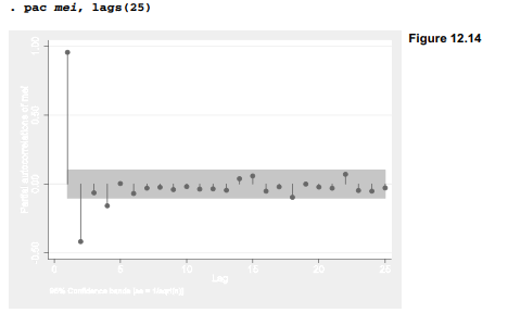
. ac mei, lags(25)

The resulting correlogram, Figure 12.13, includes a shaded area marking pointwise 95% confidence intervals. Correlations outside of these intervals are individually significant. The lags(25) option extends this graph to a 25-month lag, revealing that autocorrelations of mei become negative after about 12 months. This pattern reflects the quasi-oscillatory character of ENSO: high periods have some tendency to be followed by low ones, and vice versa.

A similar command, pac, produces the graph of partial autocorrelations in Figure 12.14. Approximate confidence intervals are based on standard error estimates of 1/v’rT . The partial autocorrelations of mei, unlike the autocorrelations, cut offto mostly nonsignificant values after a 2-month lag.

Cross-correlograms help to explore relationships between two time series. Figure 12.15 shows the cross-correlogram of Total Solar Irradiance (tsil) and mei. The cross-correlations are near zero for negative lags, and gradually become stronger (though still weak) at longer positive lags. There is virtually no correlation within the same year.

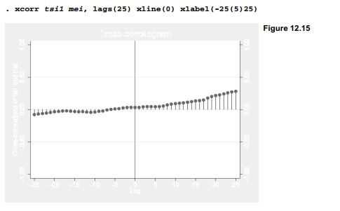
Cross-correlograms are easiest to read if we list our input or independent variable first in the xcorr command, and the output or dependent variable second—as done for Figure 12.15. Then positive lags denote correlations between input at time t and output at time t +1, t +2 etc. In this graph we see some correlation between solar irradiance and the state of ENSO about two years later, consistent with a mild, delayed solar influence on ENSO. There is no correlation between solar irradiance and the state of ENSO two years earlier, giving (sensibly) no reason to think that ENSO affects the sun.

The actual cross-correlation coefficients, and a text version of the cross-correlogram, can be obtained with the table option:

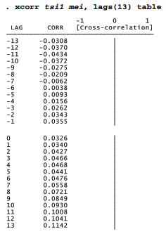
The remainder of this chapter goes beyond correlation to more formal time series modeling.

Source: Hamilton Lawrence C. (2012), Statistics with STATA: Version 12, Cengage Learning; 8th edition.