Missing Value Codes in Stata

Examples seen so far involve only a single missing-value code, Stata’s default: a large number which Stata displays as a period. In some datasets, however, values might be missing for several different reasons. We could denote different kinds of missing values by using extended missing- value codes. These are even larger numbers, which Stata displays as “.a” through “.z”. Unlike the default missing-value code “.”, the extended missing-value codes can be labeled.

Different kinds of missing values often arise with surveys, where the question “In what year were you married?” might have no answer because the respondent has never been married, can’t recall, or thinks it’s none of your business. Dataset Granite2011_6.dta, contains data from a political opinion survey, New Hampshire’s Granite State Poll. A question asking respondents about their level of interest regarding the 2012 general election (genint) serves to illustrate Stata’s extended missing-value codes.

At first glance, genint appears straightforward, but for many analyses this variable would be awkward to use.

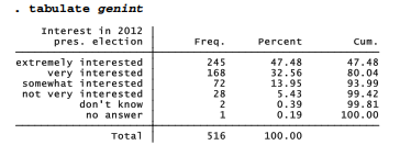
The first four values, labeled “extremely interested” to “not very interested” form a scale of disinterest. The last two, “don’t know” and “no answer” are not part of this scale but two different kinds of non-answers. Like many other surveys, the Granite State Poll employs particular numbers to represent various non-answers. In this case, the number 98 means the respondent said he or she did not know how interested they were, and 99 means no answer was given. We can see these numerical values if we ask for the same table without value labels.

Any statistics calculated for genint will be confused by the 98 and 99 codes. For example, a table of genint means by respondent education will be meaningless, because those 98 and 99 values have been averaged in.

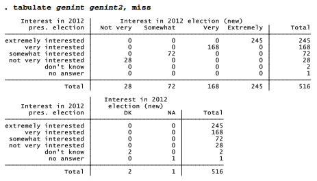
We need an improved version of this variable, to be called genint2. This new version will be different in three ways. First, we reverse the 1 through 4 values so that higher values indicate greater interest instead of less interest — making interpretation more natural.

. generate genint2 = 5 – genint if genint <90

Second, the 98 and 99 values should be identified as missing so they do not enter calculations for the mean and other statistics. Here we use the missing value code .a to represent “don’t know” responses, formerly coded 98. We use .b to represent “no answer” responses, formerly coded 99.

. replace genint2 = .a if genint == 98

. replace genint2 = .b if genint == 99

Third, the value labels can be shortened from long phrases like “extremely interested” to something that will take up less space in graphs and tables.

. label variable genint2 “Interest in 2012 election (new)”

. label define genint2 1 “Not very” 2 “Somewhat” 3 “Very” 4 “Extremely”  .a  “DK” .b “NA”

. label values genint2 genint2

Finally, a very important step: tabulating old against new variables to be sure that our commands worked as intended.

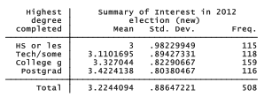
With these changes we have a more analyzable version. For example, it is easy to see that the average level of interest in the election rises with education.

. tabulate educ, summ(genint2)

Any time we encounter specific numbers (such as 98 and 99 in the example above) used to indicate missing values, it is advisable to change these to missing value codes so that Stata does not enter the fake numbers into statistical calculations. This could be done easily for a whole list of variables using an mvdecode command such as

. mvdecode genint income age, mv(97=. \ 98=.a \ 99=.b)

The example above would change any values of genint, income or age from 97 to “.”, from 98 to “.a” and so forth. The .a and .b (through .z) missing values can accept value labels, but “.” by itself cannot.

As usual, the changes we have made do not become permanent until our dataset is saved. After so much recoding, it makes sense to save these data with a new name — in case, for some future reason, we want to take another look at the original raw data.

Source: Hamilton Lawrence C. (2012), Statistics with STATA: Version 12, Cengage Learning; 8th edition.