Individual Demand

This section shows how the demand curve of an individual consumer follows from the consumption choices that a person makes when faced with a budget constraint. To illustrate these concepts graphically, we will limit the avail- able goods to food and clothing, and we will rely on the utility-maximization approach described in Section 3.3 (page 86).

1. Price Changes

We begin by examining ways in which the consumption of food and cloth- ing changes when the price of food changes. Figure 4.1 shows the consump- tion choices that a person will make when allocating a fixed amount of income between the two goods.

Initially, the price of food is $1, the price of clothing $2, and the consum- er ’s income $20. The utility-maximizing consumption choice is at point B in Figure 4.1 (a). Here, the consumer buys 12 units of food and 4 units of clothing, thus achieving the level of utility associated with indifference curve U2.

Now look at Figure 4.1 (b), which shows the relationship between the price of food and the quantity demanded. The horizontal axis measures the quantity of food consumed, as in Figure 4.1 (a), but the vertical axis now measures the price of food. Point G in Figure 4.1 (b) corresponds to point B in Figure 4.1 (a). At G, the price of food is $1, and the consumer purchases 12 units of food.

Suppose the price of food increases to $2. As we saw in Chapter 3, the budget line in Figure 4.1 (a) rotates inward about the vertical intercept, becoming twice as steep as before. The higher relative price of food has increased the magnitude of the slope of the budget line. The consumer now achieves maximum utilityat A,  which is found on a lower indifference curve, U1. Because the price of food has risen, the consumer ’s purchasing power—and thus attainable utility—has fallen. At A, the consumer chooses 4 units of food and 6 units of clothing. In Figure 4.1 (b), this modified consumption choice is at E, which shows that at a price of $2, 4 units of food are demanded.

Finally, what will happen if the price of food decreases to 50 cents? Because the budget line now rotates outward, the consumer can achieve the higher level of utility associated with indifference curve U3 in Figure 4.1 (a) by selecting D, with 20 units of food and 5 units of clothing. Point H in Figure 4.1 (b) shows the price of 50 cents and the quantity demanded of 20 units of food.

2. The Individual Demand Curve

We can go on to include all possible changes in the price of food. In Figure 4.1 (a), the price-consumption curve traces the utility-maximizing combinations of food and clothing associated with every possible price of food. Note that as the price of food falls, attainable utility increases and the consumer buys more food. This pattern of increasing consumption of a good in response to a decrease in price almost always holds. But what happens to the consumption of clothing as the price of food falls? As Figure 4.1 (a) shows, the consumption of clothing may either increase or decrease. The consumption of both food and clothing can increase because the decrease in the price of food has increased the consumer ’s ability to purchase both goods.

An individual demand curve relates the quantity of a good that a single consumer will buy to the price of that good. In Figure 4.1 (b), the individual demand curve relates the quantity of food that the consumer will buy to the price of food. This demand curve has two important properties:

1. The level of utility that can be attained changes as we move along the

The lower the price of the product, the higher the level of utility. Note from Figure 4.1 (a) that a higher indifference curve is reached as the price falls. Again, this result simply reflects the fact that as the price of a product falls, the consumer ’s purchasing power increases.

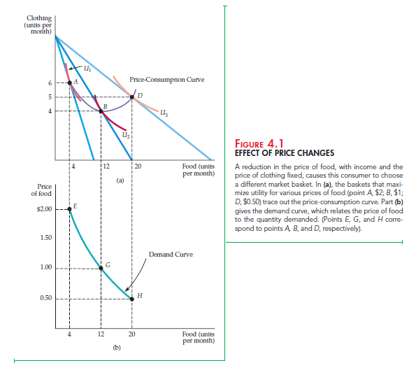
for clothing equals the ratio of the prices of food and clothing. As the price of food falls, the price ratio and the MRS also fall. In Figure 4.1 (b), the price ratio falls from 1 ($2/$2)  at E (because the curve U1  is tangent to a budget line with a slope of -1 at A) to 1/2  ($1/$2) at G, to 1/4  ($0.50/$2) at H. Because the con- sumer is maximizing utility, the MRS of food for clothing decreases as we move down the demand curve. This phenomenon makes intuitive sense because it tells us that the relative value of food falls as the consumer buys more of it.

The fact that the MRS varies along the individual’s demand curve tells us something about how consumers value the consumption of a good or service. Suppose we were to ask a consumer how much she would be willing to pay for an additional unit of food when she is currently consuming 4 units. Point E on the demand curve in Figure 4.1 (b) provides the answer: $2. Why? As we pointed out above, because the MRS of food for clothing is 1 at E, one additional unit of food is worth one additional unit of clothing. But a unit of clothing costs $2, which is, therefore, the value (or marginal benefit) obtained by consuming an additional unit of food. Thus, as we move down the demand curve in Figure 4.1 (b), the MRS falls. Likewise, the value that the consumer places on an addi- tional unit of food falls from $2 to $1 to $0.50.

3. Income Changes

We have seen what happens to the consumption of food and clothing when the price of food changes. Now let’s see what happens when income changes.

The effects of a change in income can be analyzed in much the same way as a price change. Figure 4.2 (a) shows the consumption choices that a consumer will make when allocating a fixed income to food and clothing when the price of food is $1 and the price of clothing $2. As in Figure 4.1 (a), the quantity of clothing is measured on the vertical axis and the quantity of food on the horizontal axis. Income changes appear as changes in the budget line in Figure 4.2 (a). Initially, the consumer ’s income is $10. The utility-maximizing consumption choice is then at A, at which point she buys 4 units of food and 3 units of clothing.

This choice of 4 units of food is also shown in Figure 4.2 (b) as E on demand curve D1. Demand curve D1  is the curve that would be traced out if we held income fixed at $10 but varied the price of food. Because we are holding the price of food constant, we will observe only a single point E on this demand curve.

What happens if the consumer ’s income is increased to $20? Her budget line then shifts outward parallel to the original budget line, allowing her to attain the utility level associated with indifference curve U2. Her optimal consump- tion choice is now at B, where she buys 10 units of food and 5 units of clothing. In Figure 4.2 (b) her consumption of food is shown as G on demand curve D2. D2  is the demand curve that would be traced out if we held income fixed at $20 but varied the price of food. Finally, note that if her income increases to $30, she chooses D, with a market basket containing 16 units of food (and 7 units of clothing), represented by H in Figure 4.2 (b).

We could go on to include all possible changes in income. In Figure 4.2 (a), the income-consumption curve traces out the utility-maximizing combina- tions of food and clothing associated with every income level. The income- consumption  curve  in  Figure  4.2  slopes  upward  because  the  consump- tion of both food and clothing increases as income increases. Previously, we saw that a change in the price of a good corresponds to a movement along a demand curve. Here, the situation is different. Because each demand curve is

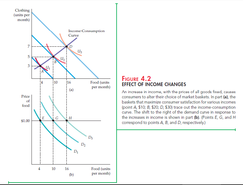
measured for a particular level of income, any change in income must lead to a shift in the demand curve itself. Thus A on the income-consumption curve in Figure 4.2 (a) corresponds to E on demand curve D1   in Figure 4.2 (b); B corresponds to G on a different demand curve D2. The upward-sloping income-consumption curve implies that an increase in income causes a shift to the right in the demand curve—in this case from D1 to D2 to D3.

4. Normal versus Inferior Goods

When the income-consumption curve has a positive slope, the quantity demanded increases with income. As a result, the income elasticity of demand is positive. The greater the shifts to the right of the demand curve, the larger the income elasticity. In this case, the goods are described as normal: Consumers want to buy more of them as their incomes increase.

In some cases, the quantity demanded falls as income increases; the income elasticity of demand is negative. We then describe the good as inferior. The term inferior simply means that consumption falls when income rises. Hamburger, for example, is inferior for some people: As their income increases, they buy less hamburger and more steak.

Figure 4.3 shows the income-consumption curve for an inferior good. For relatively low levels of income, both hamburger and steak are normal goods. As income rises, however, the income-consumption curve bends backward (from point B to C). This shift occurs because hamburger has become an inferior good—its consumption has fallen as income has increased.

5. Engel Curves

Income-consumption curves can be used to construct Engel curves, which relate the quantity of a good consumed to an individual’s income. Figure 4.4 shows how such curves are constructed for two different goods. Figure 4.4 (a), which shows

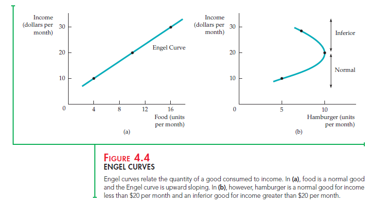
an upward-sloping Engel curve, is derived directly from Figure 4.2 (a). In both figures, as the individual’s income increases from $10 to $20 to $30, her consump- tion of food increases from 4 to 10 to 16 units. Recall that in Figure 4.2 (a) the verti- cal axis measured units of clothing consumed per month and the horizontal axis units of food per month; changes in income were reflected as shifts in the budget line. In Figures 4.4 (a) and (b), we have replotted the data to put income on the vertical axis, while keeping food and hamburger on the horizontal.

The upward-sloping Engel curve in Figure 4.4 (a)—like the upward-sloping income-consumption curve in Figure 4.2 (a)—applies to all normal goods. Note that an Engel curve for clothing would have a similar shape (clothing consump- tion increases from 3 to 5 to 7 units as income increases).

Figure 4.4 (b), derived from Figure 4.3, shows the Engel curve for hamburger. We see that hamburger consumption increases from 5 to 10 units as income increases from $10 to $20. As income increases further, from $20 to $30, con- sumption falls to 8 units. The portion of the Engel curve that slopes downward is the income range within which hamburger is an inferior good.